This answer might not be what you are expecting, but I think the concept is very useful. It's based on a previous answer of mine found here:
What is the relation between NE555 voltage doubler output voltage vs load?
Note: I would also check out the other answers on this question since it's similar to yours.
Like you said, the circuit is non-linear so it's difficult to come up with an exact answer. However, if you limit the valid range of load resistor values you can use your measurements to calculate a linear equivalent circuit where you can predict the output using a much simpler linear equation. You're basically transforming the non-linear I-V curve of the circuit to a straight-line approximation which crosses two points on the original curve. How good the approximation will be depends on the two points you select, including how close/far-apart they are and also where the points you are trying to predict are in relation to the original two points.
This is basically an application of Thévenin's theorem. You can redraw the circuit to the left of your load resistor as a voltage source and series resistor. You already have two data points from your CircuitLab simulations. The voltage with infinite load resistance and the voltage with a 10 kΩ load resistor: (\$\infty\$ Ω, 4.3 V) and (10 kΩ, 2.8 V), respectively. You can actually use a simplified version of the Thévenin calculation (shown below) due to the open-circuit voltage being equal to \$V_{th}\$. However, using this data point has some issues for your particular circuit.
$$
R_{th} = R_{L} \cdot \Big( \frac{V_{th}}{V_{out}}-1 \Big) = 10 \text{ kΩ} \cdot \Big( \frac{4.3 \text{ V}}{2.8 \text{ V}}-1 \Big) \approx 5.357 \text{ kΩ}
$$
First, the infinite load resistance causes the circuit to take a very long time to reach true steady-state. You simulated your circuit and assumed steady-state when the output got to 4.3V, but if you run it for longer you'll see that it can get even higher. For an ideal diode, it will eventually reach 5V but the 1N4148 simulation model has reverse leakage which will make it reach just shy of 5V. In real life, your multimeter's input resistance will affect the output measurement even further.
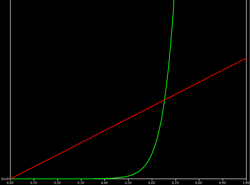
Second, if you picture a diode I-V curve, the current hangs near zero for a very wide range of low voltages. The infinite load resistance means you're taking the data point at the origin. So a linear approximation (red) made from one point at the origin and one point elsewhere on the original curve (green) will look something like below. As you can see, this is a very poor approximation.

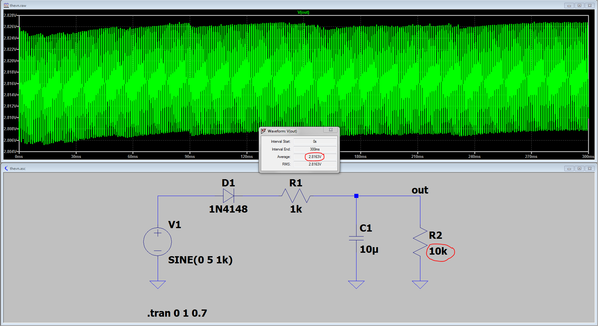
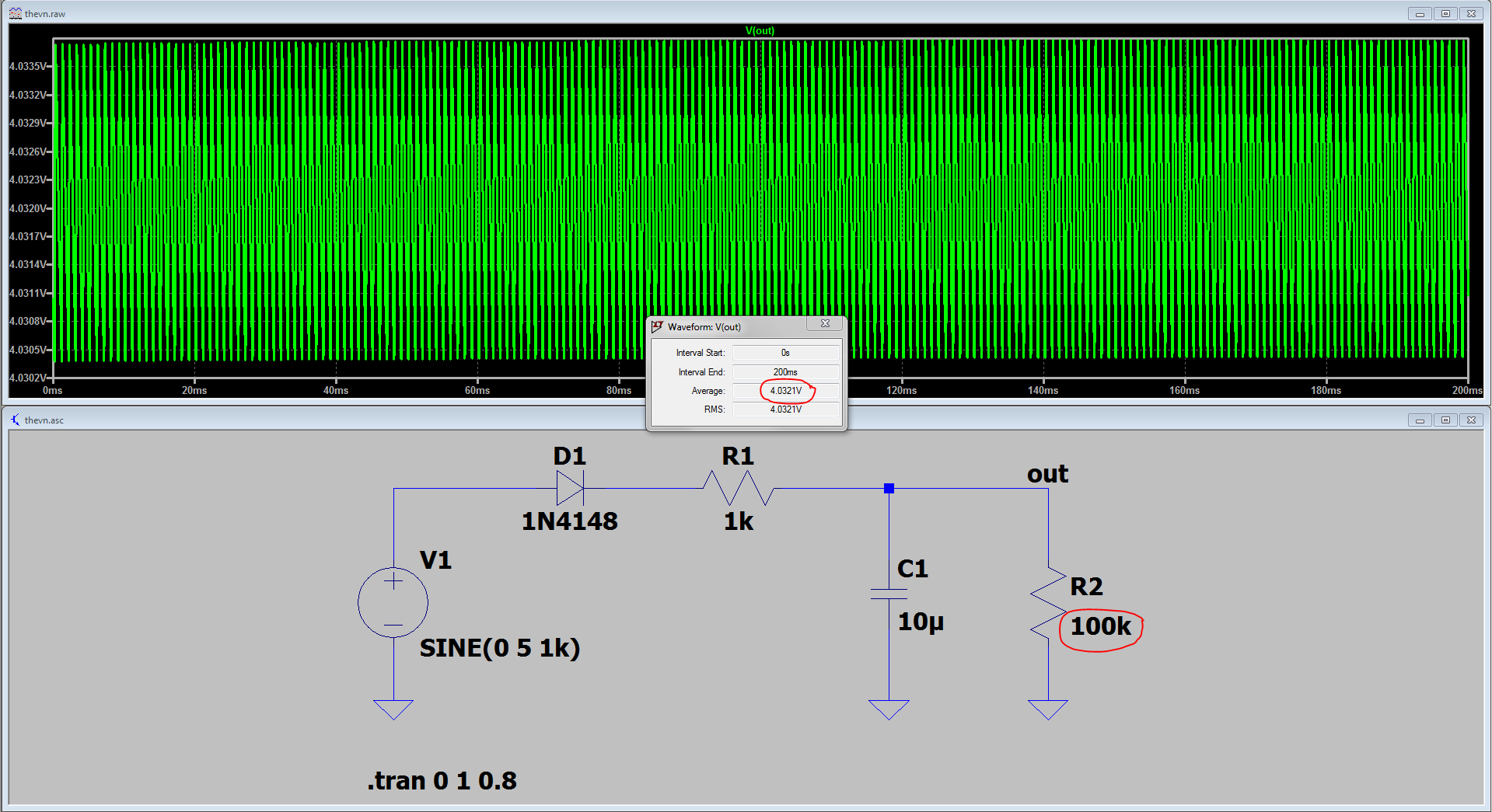
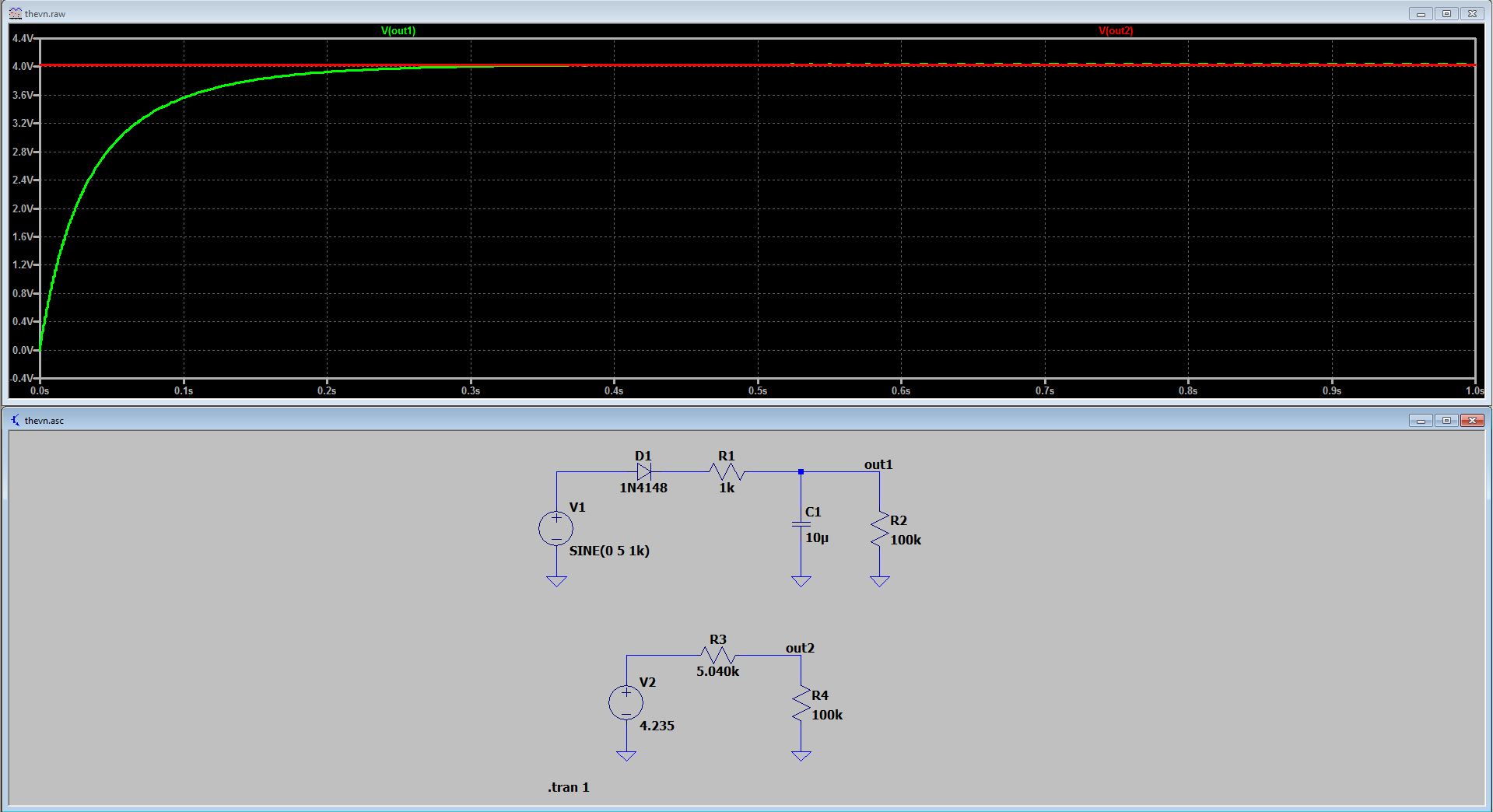
Therefore, you need to pick a more practical 2nd data point for this kind of circuit. Let's choose 100 kΩ. Simulating both 10 kΩ and 100 kΩ loads, we get the following data points for \$(R_{Lx},V_{outx})\$:
$$
\begin{align*}
(R_{L1},V_{out1}) &= (10 \text{ kΩ},2.816 \text{ V}) \\
(R_{L2},V_{out2}) &= (100 \text{ kΩ},4.032 \text{ V})
\end{align*}
$$


Using the equations from the answer I linked above, we can calculate \$R_{th}\$ and \$V_{th}\$ from these two data points.
$$
\begin{align*}
R_{th} &= \frac{R_{L1}R_{L2}(V_{out2} - V_{out1})}{V_{out1}R_{L2} - V_{out2}R_{L1}} \\~\\ R_{th} &\approx 5.040 \text{ kΩ} \\~\\ \\
V_{th} &= V_{outx} \cdot \frac{R_{th} + R_{Lx}}{R_{Lx}} \quad \text{for} \ x = 1 \ \text{or} \ 2 \\~\\ V_{th} &\approx 4.235 \text{ V}
\end{align*}
$$
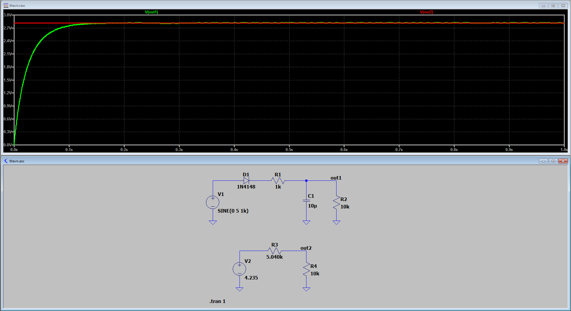
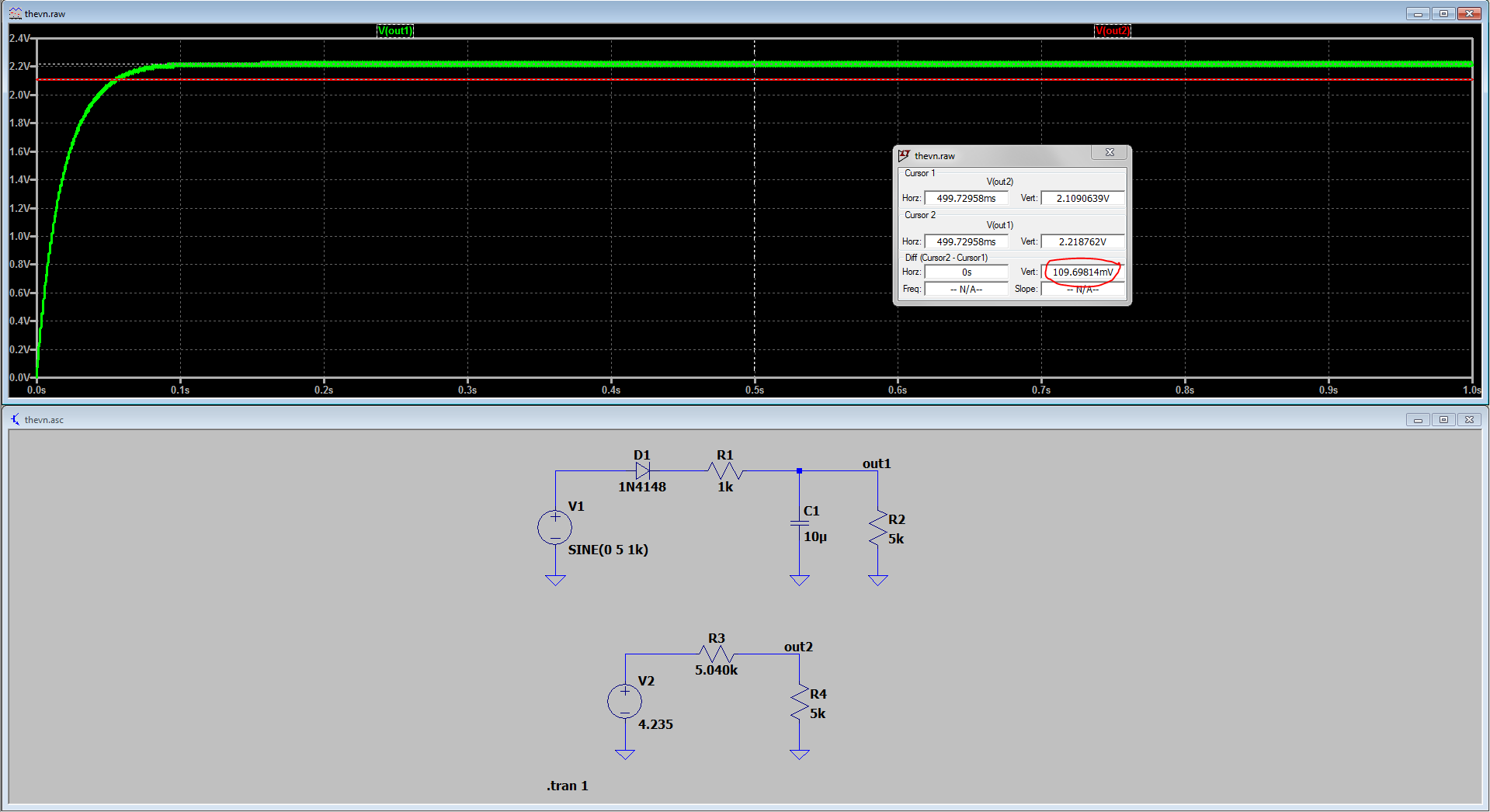
We can now compare our linearized circuit with the actual circuit and see how well our approximation does. First, we start with the points we used to construct the approximation. If we didn't make a mistake in the calculations, the approximation should match up exactly with the original circuit for 10 kΩ and 100 kΩ loads...and they do.


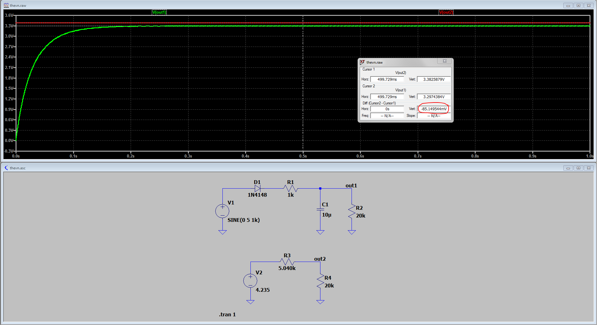
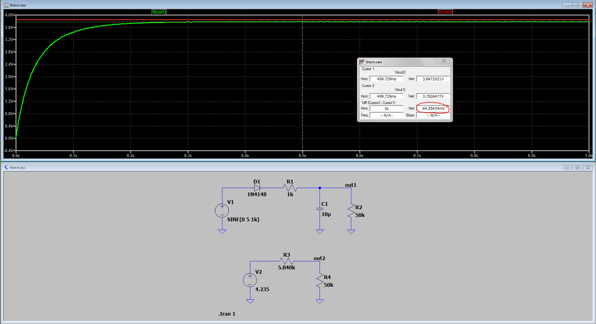
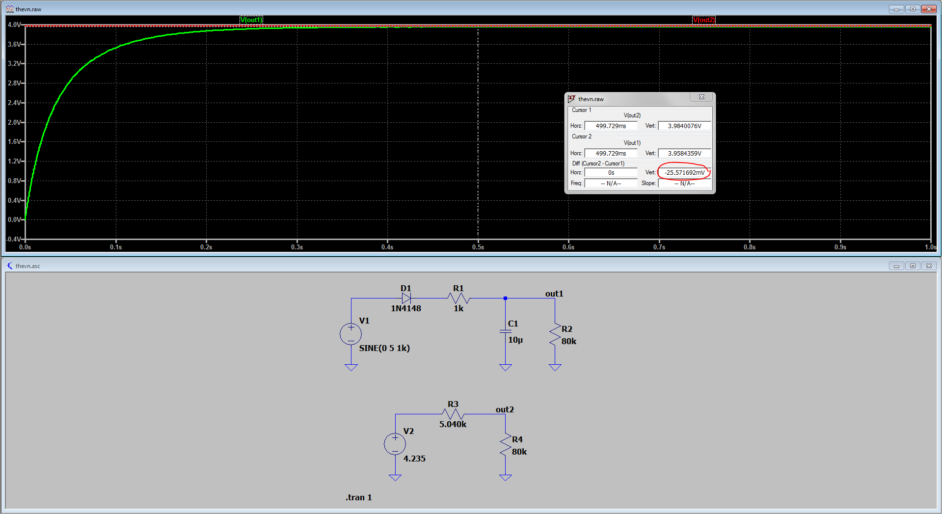
We can try some points in between to see how well the approximation fares. Let's try 20 kΩ, 50 kΩ, and 80 kΩ. I circled the voltage difference between the original and the approximation in red.


That's pretty darn close. OK, so let's try some points outside the original range of 10 kΩ to 100 kΩ. How about 5 kΩ and 200 kΩ?


A little bit worse, but still really good. OK, so this approximation can work for us reasonably well under these load conditions. So how do we use it without the simulator? Well, a Thévenin equivalent connected into a load resistor is just a simple voltage divider circuit. So for this particular circuit, we can approximate the output voltage \$V_{out}\$ given the load resistance \$R_{L}\$ as such:
$$
V_{out} \approx 4.235 \text{ V} \cdot \frac{R_L}{5.040 \text{ kΩ} + R_L}
$$
For example, for \$R_L = 68 \text{ kΩ}\$ we should get:
$$
V_{out} \approx 4.235 \text{ V} \cdot \frac{68 \text{ kΩ}}{5.040 \text{ kΩ} + 68 \text{ kΩ}} \approx 3.943 \text{ V}
$$
This technique can be very useful if utilized properly while understanding its limitations. The better you can place your two data points with respect to your intended operating condition range will determine how accurate your approximation can be over that range. In the real world, you can use this scheme to measure and characterize unknown circuits, such as the output pin of an integrated circuit. Take two load resistor measurements on the bench which you can then use to construct a fairly reasonable approximation (in many cases). See the answer I linked above for more details.
One last thing to mention for completeness. If you know your calculus, a straight line intersecting a function at two points is known as a secant line. As these points move closer together such that they are almost on top of each other results in what we call a tangent line. You can apply a similar concept here. If you need a really good approximation for a 10kΩ load (not a range), you can pick the 10 kΩ point and something like a 10.1 kΩ point for your calculations. Then the resulting approximation will be very good around 10kΩ, but nowhere else. The limiting factor for this kind of calculation will depend on how good the SNR and precision are for your measurement equipment. If the resulting measured voltage for the 10.1 kΩ load is not much different than the 10 kΩ load, then you might need to try something like 10.5 kΩ or 11.0 kΩ.

