I'm using a Tektronix TDS 1002B oscilloscope. I was investigating some glitch issues on pulses/square-waves and decided to save the time-series data to a USB drive in CSV file format to plot in MATLAB.
Input to the scope is a square-wave or pulse.
When I set the scope's Acquire feature to 'Peak Detect' setting, and observe the signal on the scope's screen live I only see over-shootings at the rising edges but the pulse seems it has no glitches. But then I save this signal data(using Save feature) to a USB drive in CSV file format to plot in MATLAB.
In the following example, the input to the scope is a 50Hz 4Vpp square-wave.
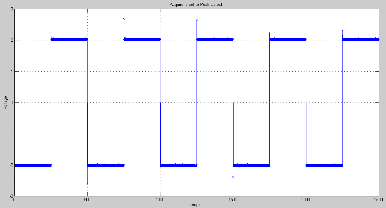
When I set the Acquire to 'Peak Detect' and saved the data in CSV format, here is what I plot in MATLAB:
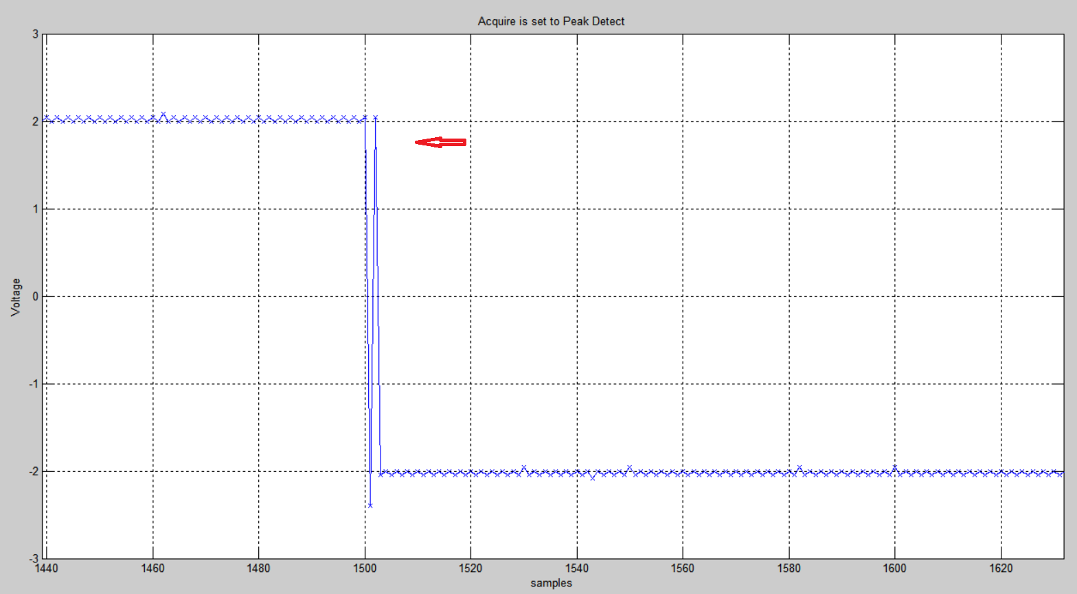
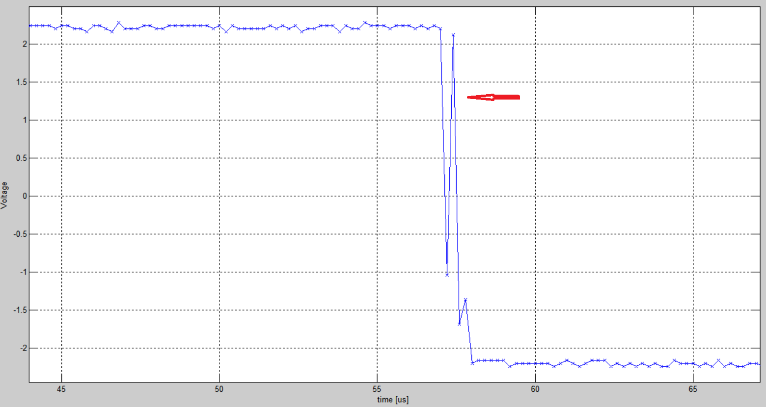
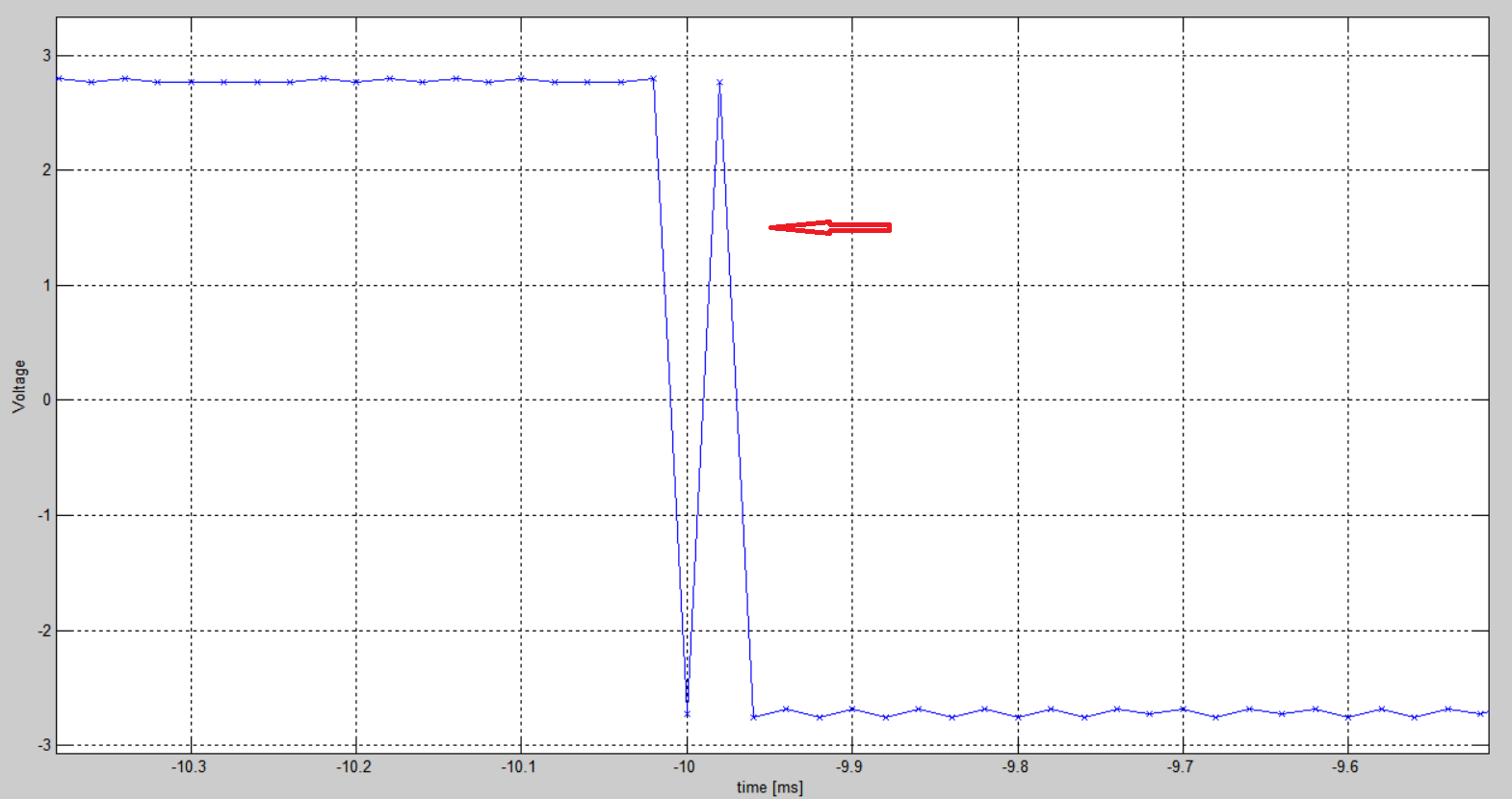
And here in the zoomed view I see glitch on each falling edge:
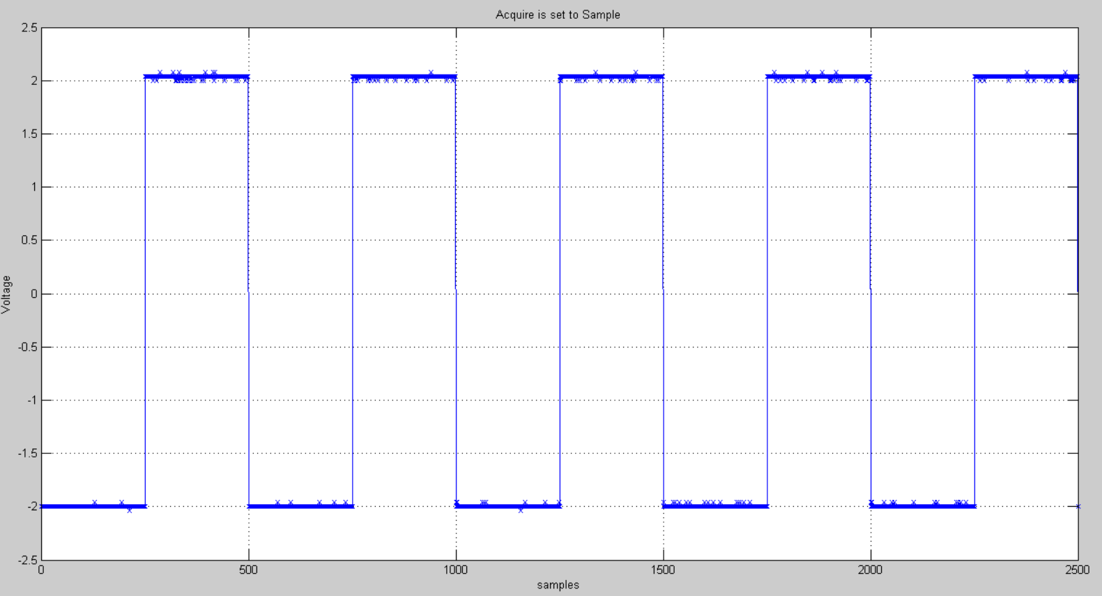
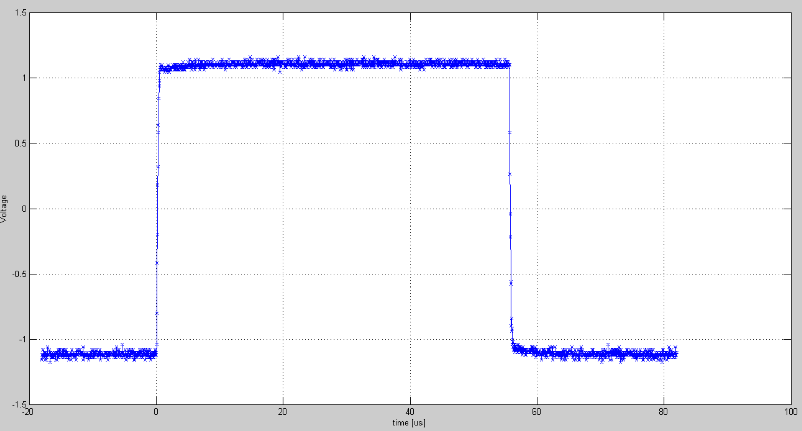
On the other hand, when I set the Acquire to 'Sample' and saved the data in CSV format, here is what I plot in MATLAB:
As you see the square-wave is clean and free of glitches:
I tested this measurement with different inputs I mean different function generators and pulse outputting devices at various frequencies. But I always see same type of glitch always on the falling edges when the Acquire is set to 'Peak Detect' and saved as in CSV format.
I made the same test with a chinese scope Siglent SDS1102CML and when I saved the data in Peak Detect mode I don't see any glitches.
What would the reason be for those glitches after each falling edge. Is that an oscilloccope error?
Edit:
Following PlasmaHH's advice I checked the measuremtns with more horizontal settings. When I decrease the division enough, at some point the saved data for falling edges are clean, glitches disappear.
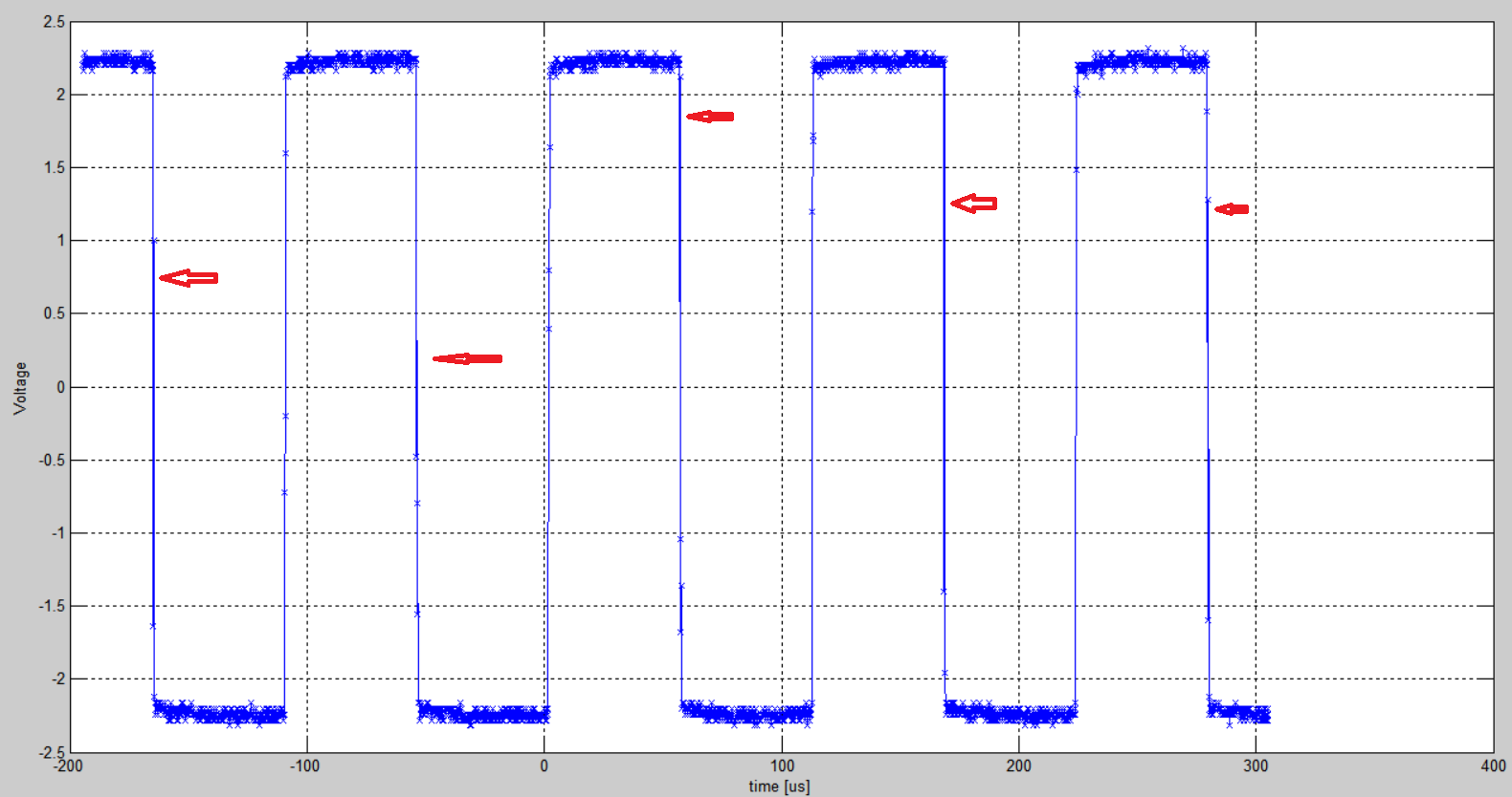
When the horizontal is set to 50us here is the data saved:
And here is the zoomed view of a glitchy falling edge:
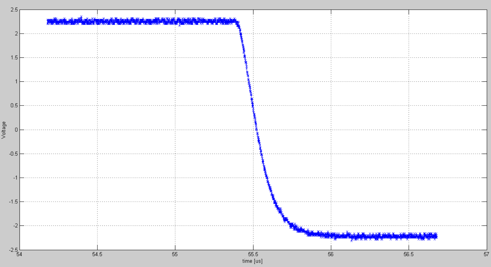
When the horizontal is set to 5us there is no glitch, here is the data saved:
When the horizontal is set to 250ns there is no glitch, here is the data saved:
Edit 2
Horizontal is set to 5ms per division. The input is 50Hz square wave.
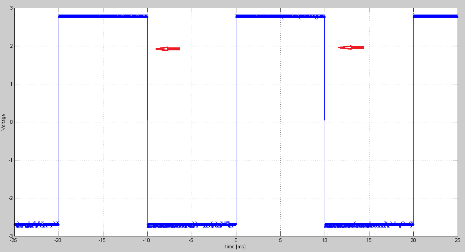
Here are the results:
Each falling edge has glitch. And here is the zoomed view:
And here below is the data from CSV file where the first glitch occurs:
t = [-0.01006 -0.01004 -0.01002 -0.01 -0.00998 -0.00996 -0.00994 -0.00992 -0.0099 -0.00988 -0.00986 -0.00984 ];
V= [2.76 2.76 2.8 -2.72 2.76 -2.76 -2.68 -2.76 -2.68 -2.76 -2.68 -2.76 ]
plot(t,V)

