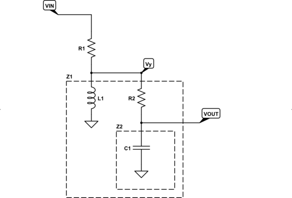
Your schematic is as follows:

simulate this circuit – Schematic created using CircuitLab
Above, you can see that \$R_2\$ and \$Z_2\$ form a voltage divider that divides \$V_Y\$ into \$V_\text{OUT}\$. It follows that:
$$\begin{align*}
\text{Each Stage}
\left\{
\begin{array}{rl}
V_\text{OUT} = V_Y\,\frac{1}{1+\frac{R_2}{Z_2}}&&Z_2 = \left(Z_{C_1}\mid\mid \infty\right)=Z_{C_1}\\\\
V_Y = V_\text{IN}\,\frac{1}{1+\frac{R_1}{Z_1}}&&Z_1 = Z_{L_1}\mid\mid \left(Z_2 + R_2\right)
\end{array}
\right.
\end{align*}$$
$$\therefore \frac{V_\text{OUT}}{V_\text{IN}}=\frac{1}{1+\frac{R_1}{Z_1}}\cdot\frac{1}{1+\frac{R_2}{Z_2}}$$
From that, I get:
$$H\left(s\right)=\frac{L_1\,s}{L_1\,C_1\left(R_1+R_2\right)s^2+\left(R_1\,R_2\,C_1+L_1\right)s+R_1}$$
That is not in standard form, though. To get started, you want to divide through so that you isolate \$s^2\$ in the denominator. So, something like this to start:
$$H\left(s\right)=\frac{\frac{1}{C_1\left(R_1+R_2\right)}\,s}{s^2+\frac{R_2\,C_1+\frac{L_1}{R_1}}{L_1\,C_1\left(1+\frac{R_2}{R_1}\right)}\,s+\frac{1}{L_1\,C_1\left(1+\frac{R_2}{R_1}\right)}}$$
Set \$\alpha=\frac12\cdot \frac{R_2\,C_1+\frac{L_1}{R_1}}{L_1\,C_1\left(1+\frac{R_2}{R_1}\right)}\$, \$\omega_{_0}=\frac{1}{\sqrt{L_1\,C_1\left(1+\frac{R_2}{R_1}\right)}}\$, and create the unitless damping factor of \$\zeta=\frac{\alpha}{\omega_{_0}}\$.
The standard form for a 2nd order bandpass is:
$$H\left(s\right)=K\cdot \frac{2\zeta\,\omega_{_0}\,s}{s^2+2\zeta\,\omega_{_0}\,s+\omega_{_0}^2}$$
Where \$K\$ is the voltage gain. You can now solve for \$K\$.
It may be convenient to set \$\tau_{_1}=\frac{L_1}{R_1}\$ and \$\tau_{_2}=R_2\,C_1\$.
Then you should find:
$$K=\frac{1}{1+\frac{\tau_{_2}}{\tau_{_1}}}$$
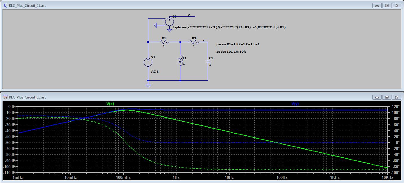
With all values set to 1, as you show, this means \$K=\frac12\$ or \$-6\;\text{dB}\$.
Let's re-examine \$H\left(s\right)\$ with some light from above.
We know that \$\omega_{_0}\cdot \tau_{_0}=1\$, so it follows that: \$\tau_{_0}=\sqrt{L_1\,C_1\left(1+\frac{R_2}{R_1}\right)}\$
Let's follow through with some algebra and replacements:
$$\begin{align*}
H\left(s\right)&=\frac{\frac{1}{C_1\left(R_1+R_2\right)}\,s}{s^2+\frac{R_2\,C_1+\frac{L_1}{R_1}}{L_1\,C_1\left(1+\frac{R_2}{R_1}\right)}\,s+\frac{1}{L_1\,C_1\left(1+\frac{R_2}{R_1}\right)}}\\\\
&=\frac{\frac{\frac{L_1}{R_1}}{L_1\,C_1\left(1+\frac{R_2}{R_1}\right)}\,s}{s^2+\frac{R_2\,C_1+\frac{L_1}{R_1}}{L_1\,C_1\left(1+\frac{R_2}{R_1}\right)}\,s+\frac{1}{L_1\,C_1\left(1+\frac{R_2}{R_1}\right)}}\\\\
&=\frac{\tau_{_1}\,\omega_{_0}^2\,s}{s^2+\left(\tau_{_1}+\tau_{_2}\right)\omega_{_0}^2\,s+\omega_{_0}^2}
\end{align*}$$
From this, we can fathom that the damping factor is \$\zeta=\frac12\,\left(\tau_{_1}+\tau_{_2}\right)\omega_{_0}\$. (Look back at the definitions for \$\alpha\$, \$\omega_{_0}\$, and \$\zeta\$ earlier above.)
Looking only at the numerator now, we know that \$K\,2\zeta\,\omega_{_0}=K\,2\left(\frac12\,\left(\tau_{_1}+\tau_{_2}\right)\omega_{_0}\right)\,\omega_{_0}=\tau_{_1}\,\omega_{_0}^2\$ or that \$K\left(\tau_{_1}+\tau_{_2}\right)=\tau_{_1}\therefore K=\frac{\tau_{_1}}{\tau_{_1}+\tau_{_2}}=\frac{1}{1+\frac{\tau_{_2}}{\tau_{_1}}}\$
Q.E.D.
I hadn't realized you wanted the branch current through \$R_2\$ and \$C_1\$ divided by \$V_\text{IN}\$, before. But everything is present above to develop it. Take the equation for \$V_Y\$ from above and divide it by the branch impedance, \$R_2+Z_{C_1}\$:
$$\begin{align*}
I&=\frac{V_Y}{R_2+Z_{C_1}} = V_\text{IN}\,\frac{1}{1+\frac{R_1}{Z_1}}\,\frac{1}{R_2+Z_{C_1}}\\\\&\therefore\\\\
\frac{I}{V_\text{IN}}&=\frac{L_1\,C_1\,s^2}{L_1\,C_1\left(R_1+R_2\right)s^2+\left(R_1\,R_2\,C_1+L_1\right)s+R_1}
\end{align*}$$
But the easier way to see the above result is to just go back to your \$\frac{V_\text{OUT}}{V_\text{IN}}\$ transfer function. \$V_\text{OUT}\$ is riding on top of \$C_1\$. So the branch current is \$I=\frac{V_\text{OUT}}{Z_2}\$. All you have to do is:
$$\frac{I}{V_\text{IN}}=\frac{V_\text{OUT}}{V_\text{IN}}\cdot \frac{I}{V_\text{OUT}}=\frac{V_\text{OUT}}{V_\text{IN}}\cdot\frac1{Z_2}=\frac{V_\text{OUT}}{V_\text{IN}}\cdot \bigg[C_1\, s\bigg]$$
Nothing at all difficult to see.
Final note to OP on using sympy for problems such as the above
Since you expressed an interest in sympy (which I most certainly recommend to you), I'll disclose below what I did to save myself time (and mindless mistakes) when creating the equations I used above.
(I also recommend including a numeric solver, SageMath. I use Sage with sympy, myself. Be sure to google around to see how others have installed both on your operating system of choice.)
I entered the following, to get started:
var('vin vout vy l1 c1 r1 r2 s')
z2=1/s/c1
z1=(s*l1)*(z2+r2)/(s*l1+z2+r2)
hs=simplify(1/(1+r1/z1)/(1+r2/z2))
Then I write the first line below, which printed out the second line:
hs
l1*s/(l1*s*(c1*r2*s + 1) + r1*(c1*s*(l1*s + r2) + 1))
Well, sympy has its own style of generating "best output" by factoring things. I didn't like it much, so I wrote something to just grab the denominator, expand it (un-factor it) out, and then factor it back over 's', instead. The first line is what I wrote; the second line is what it gave back:
factor(expand(fraction(hs)[1]),s)
r1 + s**2*(c1*l1*r1 + c1*l1*r2) + s*(c1*r1*r2 + l1)
Now, that looks a lot better.
Pretty easy, right??
But then I wanted "standard form." So now the following (a is \$\alpha\$, w0 is \$\omega_{_0}\$, etc):
a=(r1*r2*c1+l1)/2/l1/c1/(r1+r2)
w0=sqrt(r1/l1/c1/(r1+r2))
zeta=a/w0
I knew that \$K=\frac{H\left(s\right)}{\left[\frac{2\zeta\,\omega_{_0}\,s}{s^2+2\zeta\,\omega_{_0}\,s+\omega_{_0}^2}\right]}\$, so I added:
K=simplify(hs/((2*zeta*w0*s)/(s**2+2*zeta*w0*s+w0*w0)))
To see what that was:
K
l1/(c1*r1*r2 + l1)
Well, this immediately told me something important. Divide top and bottom by \$L_1\$ and I get: \$\frac{1}{1+\frac{R_2\,C_1}{\frac{L_1}{R_1}}}\$. (The denominator is unitless, as it must be. And so I kept both factors in terms of time so that the unit cancellation was obvious. )
That's probably enough for now. You get the idea. It's really easy!
Sage, if you use it, has its own "shell variable" called "SAGE_STARTUP_FILE" which you can set to some file. When you start Sage from a shell command, it will load that file and execute the lines as if you typed them. Saves time. In my case, to get the bits of sympy I often use, my file starts this way:
%colors linux
from sympy import *
from sympy.solvers import solve
from sympy import radsimp, signsimp
from sympy.simplify.radsimp import collect_sqrt
Because it's easy to do and because I sometimes want to look at different Butterworth filters without having to go find a manual on it, I add these lines, as well:
def Butterworth(n):
    r = solve( 1+(-1)**n*x**(2*n), x )
    t = []
    for a in r:
        if real( a ) < 0:
            t.append( a )
    t.sort( key = lambda tup: real( tup ) )
    u = []
    var( 's' )
    if ( len( t ) - 2*int( len( t ) / 2 ) ) == 1:
        u.append( s + 1 )
        t.pop( 0 )
    for i in range( len( t ) / 2 ):
        scnd = collect(expand((s - t[2*i])*(s - t[2*i+1])), I, evaluate=False)[1]
        n, d = fraction( scnd )
        co = [collect_sqrt( simplify( r ) ) for r in Poly( n, s ).all_coeffs()]
        spwr = simplify( s**(len( co )-1) )
        ufactor = 0
        for j in co:
            ufactor = ufactor + spwr * factor( j/d )
            spwr = simplify( spwr/s )
        u.append( ufactor )
    return u
This allows me to write:
for x in Butterworth(2): simplify(x)
s**2 + sqrt(2)*s + 1
If I want the numbers, instead, then:
for x in Butterworth(2): simplify(x.n())
s**2 + 1.4142135623731*s + 1.0
Let's try something a little higher order, done both with irrationals as well as just approximate real numbers:
for x in Butterworth(4): simplify(x)
s**2 + s*(sqrt(4 - 2*sqrt(2)) + sqrt(2*sqrt(2) + 4) + 2*sqrt(sqrt(2) + 2))/4 + 1
s**2 + s*(-sqrt(4 - 2*sqrt(2)) + 2*sqrt(2 - sqrt(2)) + sqrt(2*sqrt(2) + 4))/4 + 1
for x in Butterworth(4): simplify(x.n())
s**2 + 1.84775906502257*s + 1.0
s**2 + 0.765366864730179*s + 1.0
Ah! But I wanted a 12th order Butterworth:
for x in Butterworth(12): simplify(x.n())
s**2 + 1.98288972274762*s + 1.0
s**2 + 1.84775906502257*s + 1.0
s**2 + 1.58670668058247*s + 1.0
s**2 + 1.21752285801744*s + 1.0
s**2 + 0.765366864730179*s + 1.0
s**2 + 0.261052384440103*s + 1.0
Well, I'm insane now. I'm going to design myself a 23rd order Butterworth filter because... well because I can:
for x in Butterworth(23): simplify(x.n())
s + 1.0
s**2 + 1.98137189207266*s + 1.0
s**2 + 1.9258345746956*s + 1.0
s**2 + 1.83442260301091*s + 1.0
s**2 + 1.70883880909298*s + 1.0
s**2 + 1.55142258140884*s + 1.0
s**2 + 1.36510628643731*s + 1.0
s**2 + 1.15336064422973*s + 1.0
s**2 + 0.920130075462304*s + 1.0
s**2 + 0.669759224341972*s + 1.0
s**2 + 0.406912026105268*s + 1.0
s**2 + 0.136484826729342*s + 1.0
Now, do you know where I can find the constants for a 23rd order Butterworth? (If so, I'll just use this: "for x in Butterworth(100): simplify(x.n())" and push up the ante a bit.)
In short, you can develop your own functions and solutions for a variety of electronic needs. I have. Pretty much anything is at your fingertips.
I sometimes want to develop my own diode equations for various LED devices. I grab a bunch of random devices from the bag and make three measurements on each one. (I do have to use a 5-digit multimeter, or better, to get necessary precision and reasonable accuracy. I have a 6.5 digit one from HP.) In this way, I can collect up the LED parameters and examine their distributions. This tells me a lot about their manufacturer and their strategies in selling them through the supplier I bought from.
So I wrote this:
def diode():
    print( "This program uses 3 diode measurements to extract parameters." )
    print( "You will need to have taken these measurements beforehand." )
    print( "Enter each point as [ <diode current>, <diode voltage> ]." )
    print( "" )
    TA= int( input( "Enter the ambient temperature in Celsius (default is 27 C): " ) or "27" )
    print( "" )
    VT= 8.61733034e-5 * ( 273.15 + TA )
    POINTS= []
    vd, id, N, ISAT, RS= symbols( "vd id N ISAT RS" )
    for i in range(3):
        pid, pvd= input( "Enter point " + str(i) + ": " ).split()
        POINTS.append( { vd: pvd, id: pid } )
    EQS= []
    for i in range(3):
        EQS.append( Eq( POINTS[i][vd], RS*POINTS[i][id] + N*VT*ln(POINTS[i][id]) - N*VT*ISAT ) )
    print( POINTS )
    print( EQS )
    ANS= solve( EQS, [ RS, N, ISAT ] )[0]
    print( "RS   = " + str(ANS[0]) )
    print( "N    = " + str(ANS[1]) )
    print( "ISAT = " + str(exp(ANS[2])) )
This program generates the model parameters I want for any LED I have in my hand from just three distinct measurement points, \$\left(V_i, I_i\right)\$.
By the way, if you think I'm joking about 100th order Butterworth? Here it is:
for x in Butterworth(100): simplify(x.n())
s**2 + 1.99975326496332*s + 1.0
s**2 + 1.99777974992394*s + 1.0
s**2 + 1.99383466746626*s + 1.0
s**2 + 1.98792191091036*s + 1.0
s**2 + 1.98004731543312*s + 1.0
s**2 + 1.97021865230955*s + 1.0
s**2 + 1.95844562124353*s + 1.0
s**2 + 1.94473984079535*s + 1.0
s**2 + 1.9291148369156*s + 1.0
s**2 + 1.91158602959666*s + 1.0
s**2 + 1.89217071765509*s + 1.0
s**2 + 1.87088806165973*s + 1.0
s**2 + 1.84775906502257*s + 1.0
s**2 + 1.82280655327089*s + 1.0
s**2 + 1.79605515152123*s + 1.0
s**2 + 1.76753126017739*s + 1.0
s**2 + 1.73726302887638*s + 1.0
s**2 + 1.70528032870818*s + 1.0
s**2 + 1.67161472273654*s + 1.0
s**2 + 1.63629943485005*s + 1.0
s**2 + 1.59936931697418*s + 1.0
s**2 + 1.56086081467666*s + 1.0
s**2 + 1.52081193120006*s + 1.0
s**2 + 1.47926218995722*s + 1.0
s**2 + 1.43625259552638*s + 1.0
s**2 + 1.39182559318463*s + 1.0
s**2 + 1.34602502701955*s + 1.0
s**2 + 1.29889609666037*s + 1.0
s**2 + 1.25048531267141*s + 1.0
s**2 + 1.20084045065177*s + 1.0
s**2 + 1.15001050408656*s + 1.0
s**2 + 1.09804563599626*s + 1.0
s**2 + 1.0449971294319*s + 1.0
s**2 + 0.990917336864815*s + 1.0
s**2 + 0.935859628521147*s + 1.0
s**2 + 0.87987833971183*s + 1.0
s**2 + 0.823028717210218*s + 1.0
s**2 + 0.765366864730179*s + 1.0
s**2 + 0.706949687558514*s + 1.0
s**2 + 0.647834836396299*s + 1.0
s**2 + 0.588080650464608*s + 1.0
s**2 + 0.527746099930746*s + 1.0
s**2 + 0.466890727711811*s + 1.0
s**2 + 0.405574590713025*s + 1.0
s**2 + 0.343858200558819*s + 1.0
s**2 + 0.281802463875165*s + 1.0
s**2 + 0.219468622182091*s + 1.0
s**2 + 0.15691819145569*s + 1.0
s**2 + 0.0942129014192853*s + 1.0
s**2 + 0.0314146346236414*s + 1.0
Of course, that's all theoretical! Assuming a sufficiently precise VNA even existed, you might be sitting around for a long time tweaking it using its time domain function.


