7
\$\begingroup\$

Is there a software (preferably open source) where one draws a schematic, one defines input and output and the software automatically gives the transfer function (to be more specific: a symbolic expression of 's')? The schematic will be simple, just R, L and Cs, so just linear systems.

I reckon that softwares like LTspice and similar take the schematic and generate first a netlist and then write the nodal equations in matrix form. I imagine that the matrix can in theory also be a symbolic expression that can be reordered at will to finally compute the transfer function.

It seems to me a very common task but I haven't been able to find something like this. There is this related question but it's 10 years old, in this days of ubiquitous CAD and people doing wonders with software I can't imagine that nobody thought of this before.

I know that LTspice and the like can do a an AC-sweep and then using system identification tools to numerically find an approximate of the transfer function. But I would like to know if this is possible using symbolic manipulations

\$\endgroup\$
8
  • 2
    \$\begingroup\$ I do this all the time with SymPy. But I construct the equations by hand. It would be trivial to write software to develop those equations, though. I don't put in any thinking at all. I just create them "by rote process." So I know this would be very easy to do. But it appears you are asking for a product/software that already exists. And that may be out of scope here. (I can't say for sure. But it feels like you are looking for a COTS solution to me.) LTspice could certainly add a simple modification to achieve this result. I'm pretty sure of that. But you'd need the source code. \$\endgroup\$ Commented Sep 15 at 13:49
  • 1
    \$\begingroup\$ It is not open source, SYRUP package under MAPLE would do it. Certainly other software would do it also. \$\endgroup\$
    – Antonio51
    Commented Sep 15 at 13:49
  • 2
    \$\begingroup\$ You can have a look at Sapwin, it is a symbolic solver which includes a schematic capture. It's free as far as I remember. \$\endgroup\$ Commented Sep 16 at 5:35
  • 1
    \$\begingroup\$ @VerbalKint I decided to show how it can be done without having to pay a bunch of money for some software. \$\endgroup\$ Commented Sep 16 at 10:22
  • \$\begingroup\$ Check SLiCAP as well \$\endgroup\$
    – Designalog
    Commented Sep 16 at 10:22

3 Answers 3

10
\$\begingroup\$

I'll perform a few of the steps by hand, below. But the process you see here can be easily coded up in Python or any other language you prefer.

(In fact, I'll write all the code needed at the end, below. That will show just how easy it is.)

I'm going to use a circuit that is simple but also complicated enough to illustrate the details required. I don't want you to miss something important.

step 1

Use a schematic capture program (for example, LTspice performs that function) to draw out your schematic and get its netlist. Then remove any comment lines or Spice command lines from the list. This will provide a simple list of conductances of length \$N\$.

For example:
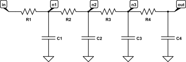
schematic

simulate this circuit – Schematic created using CircuitLab

When I put that into LTspice I get the following netlist:

R1 n1 in R
R2 n2 n1 R
R3 n3 n2 R
R4 out n3 R
C1 n1 0 C
C2 n2 0 C
C3 n3 0 C
C4 out 0 C
.backanno
.end

The last two lines aren't needed (obviously.)

This leaves a conductance list that has these \$N=8\$ elements:

R1 n1 in R
R2 n2 n1 R
R3 n3 n2 R
R4 out n3 R
C1 n1 0 C
C2 n2 0 C
C3 n3 0 C
C4 out 0 C

Should be very easy to code this up.

step 2

Scan the resulting list to create a unique list of nodes.

Do not include ground (0) in the list. It's not needed.

Also make sure that your input node is at the bottom of the list. The ordering of the rest isn't important. But that singular point of placing the input node at the bottom is important to simplify the code.

I find:

n1
n2
n3
out
in

Note again that ground is not included in the list.

This list has \$M=5\$ elements.

This will also be easily coded up. (You will need to know your input source node name, of course.)

step 3

Create an \$N\times N\$ conductance matrix, \$C\$. Each conductance is listed just once along its diagonal. Everywhere else is zero.

I'll do this manually in SymPy:

C = Matrix( [ [1/R1,0,0,0,0,0,0,0],
              [0,1/R2,0,0,0,0,0,0],
              [0,0,1/R3,0,0,0,0,0],
              [0,0,0,1/R4,0,0,0,0],
              [0,0,0,0,s*C1,0,0,0],
              [0,0,0,0,0,s*C2,0,0],
              [0,0,0,0,0,0,s*C3,0],
              [0,0,0,0,0,0,0,s*C4] ] )

Obviously easy to code since I just coded it up above, by hand. You can do this automatically given the list from step 1 and knowledge of the conductance of resistors, inductors, and capacitors.

step 4

Using the unique node list and also the simple list of conductances, create an \$N\times M\$ incidence matrix, \$A\$. This matrix starts out as all zero but will have a -1 and +1 placed on the row for each conductance found in the length-\$N\$ conductance list located at the two columns associated with the two nodes it connects.

Looking over the list from step 1 above, I get the following code:

A = Matrix( [ [-1,0,0,0,1],    # R1 n1 in R
              [1,-1,0,0,0],    # R2 n2 n1 R
              [0,1,-1,0,0],    # R3 n3 n2 R
              [0,0,1,-1,0],    # R4 out n3 R
              [-1,0,0,0,0],    # C1 n1 0 C
              [0,-1,0,0,0],    # C2 n2 0 C
              [0,0,-1,0,0],    # C3 n3 0 C
              [0,0,0,-1,0] ] ) # C4 out 0 C

That process will require re-parsing though the list from step 1. But you can see that the generation of the above isn't difficult to understand.

Note how the grounded capacitors only show one value, -1. It doesn't matter whether this is -1 or +1, as that only affects the assumed current (flux) direction. So just pick something in grounded device cases.

step 5

Now perform the following steps, using the Schur complement idea:

F = A.T * C * A               # resulting F must be square
N,M = F.shape                 # so N == M.
P = F.extract( [i for i in range(N-1)], [i for i in range(N-1)] )
QT = F.extract( [i for i in range(N-1)], [N-1] )
(-P.inv()*QT)[N-2,0]          # invert P, solve, and extract the desired transfer function.
1/(C1*C2*C3*C4*R1*R2*R3*R4*s**4 + C1*C2*C3*R1*R2*R3*s**3 + C1*C2*C4*R1*R2*R3*s**3 + C1*C2*C4*R1*R2*R4*s**3 + C1*C2*R1*R2*s**2 + C1*C3*C4*R1*R2*R4*s**3 + C1*C3*C4*R1*R3*R4*s**3 + C1*C3*R1*R2*s**2 + C1*C3*R1*R3*s**2 + C1*C4*R1*R2*s**2 + C1*C4*R1*R3*s**2 + C1*C4*R1*R4*s**2 + C1*R1*s + C2*C3*C4*R1*R3*R4*s**3 + C2*C3*C4*R2*R3*R4*s**3 + C2*C3*R1*R3*s**2 + C2*C3*R2*R3*s**2 + C2*C4*R1*R3*s**2 + C2*C4*R1*R4*s**2 + C2*C4*R2*R3*s**2 + C2*C4*R2*R4*s**2 + C2*R1*s + C2*R2*s + C3*C4*R1*R4*s**2 + C3*C4*R2*R4*s**2 + C3*C4*R3*R4*s**2 + C3*R1*s + C3*R2*s + C3*R3*s + C4*R1*s + C4*R2*s + C4*R3*s + C4*R4*s + 1)

That actually is correct, by the way. It's not in a form that will communicate well. But at least it is correct.

Note that I used \$N-2\$ as an index. This is because the output was at that position in the list from step 2. If you wanted a different transfer function, say one from \$n_2\$ for example, then all you would do is change that index.

All the answers are computed by this process. So don't use a specific index and you will get all the transfer functions at once. Or, otherwise, just pick the one you want to see (as I do, above) by specifying an index.

summary

I've demonstrated most of the directed-graph algorithmic code. All you need to do is fill in a few relatively simple blanks. However, I'll provide a complete implementation below.

Also, you may wish to read through this EESE answer to fill out a few more details.

final addition

The parsing details were interesting enough that I went ahead and wrote a quick and dirty SymPy function to handle the question:

def transfer(netlist=None,innode=None,outnode=None):
    if netlist is None:
        netlist = sys.stdin.read()
    rawlist = [i.split() for i in netlist.splitlines()]
    if len(rawlist) < 1: return 'empty netlist'
    cookedlist = []
    nodelist = []
    for i in rawlist:
        if len(i) > 2 and len(i[0]) > 1 and i[0][0].isalpha():
            device = i[0][0].upper()
            if not (device in ['R','C','L']): return 'netlist may only have R, L, or C devices'
            cookedlist.append(i[:3])
            for e in range(1,3):
                if not (i[e] == '0'): nodelist.append(i[e].upper())
    if len(cookedlist) < 1: return 'empty netlist'
    nodelist = list(set(nodelist))
    if len(nodelist) < 1: return 'enpty list of nodes'
    if innode is None or outnode is None:
        print('List of available nodes: ', ','.join(map(str, nodelist)))
        exitlist = ['', 'Q', 'E', 'QUIT', 'EXIT']
    if innode is None:
        while True:
            innode = input('Enter desired input node name: ').upper()
            if innode in nodelist: break
            if innode in exitlist: return 'user-requested termination'
            print(innode, ' not found in above list.')
    else:
        innode = innode.upper()
    if outnode is None:
        while True:
            outnode = input("Enter desired output node name (or '*' for all): ").upper()
            if outnode in nodelist: break
            if outnode == '*': break
            if outnode in exitlist: return 'user-requested termination'
            print(outnode, ' not found in above list.')
    else:
        outnode = outnode.upper()
    if not (outnode == '*'):
        temp = nodelist.pop(nodelist.index(outnode))
        nodelist.append(temp)
    temp = nodelist.pop(nodelist.index(innode))
    nodelist.append(temp)
    N = len(cookedlist)
    M = len(nodelist)
    C = zeros(N,N)
    A = zeros(N,M)
    s = symbols('s')
    for i in range(0,N):
        part = cookedlist[i][0].upper()
        device = part[0]
        partname = symbols(part, real=True, positive=True)
        if device == 'R': C[i,i] = 1/partname
        elif device == 'C': C[i,i] = s*partname
        elif device == 'L': C[i,i] = 1/(s*partname)
        else: return 'fatal internal error'
        for j in range(1,3):
            nodename = cookedlist[i][j].upper()
            if nodename == '0': continue
            if not (nodename in nodelist): return 'fatal internal error'
            nodeidx = nodelist.index(nodename)
            A[i,nodeidx] = 2*j-3
    F = A.T * C * A
    FN,FM = F.shape
    P = F.extract( [i for i in range(FN-1)], [i for i in range(FN-1)] )
    QT = F.extract( [i for i in range(FN-1)], [FN-1] )
    Answer = -P.inv()*QT
    Result = {}
    if not (outnode == '*'):
        Result[outnode] = simplify(Answer[nodelist.index(outnode),0])
    else:
        for i in range(0,M-1):
            Result[nodelist[i]] = simplify(Answer[i,0])
    return Result

It will produce just the one transfer function or all of them (when entering '*' for the output node.)

Using the above example, here's a run:

┌────────────────────────────────────────────────────────────────────┐
│ SageMath version 9.5, Release Date: 2022-01-30                     │
│ Using Python 3.10.12. Type "help()" for help.                      │
└────────────────────────────────────────────────────────────────────┘
sage: transfer()
R1 n1 vin R
R2 n2 n1 R
R3 n3 n2 R
R4 vout n3 R
C1 n1 0 C
C2 n2 0 C
C3 n3 0 C
C4 vout 0 C
.backanno
.end
List of available nodes:  N2,N3,VIN,VOUT,N1
Enter desired input node name: vin
Enter desired output node name (or '*' for all): vout
{'VOUT': 1/(C1*C2*C3*C4*R1*R2*R3*R4*s**4 + C1*C2*C3*R1*R2*R3*s**3 + C1*C2*C4*R1*R2*R3*s**3 + C1*C2*C4*R1*R2*R4*s**3 + C1*C2*R1*R2*s**2 + C1*C3*C4*R1*R2*R4*s**3 + C1*C3*C4*R1*R3*R4*s**3 + C1*C3*R1*R2*s**2 + C1*C3*R1*R3*s**2 + C1*C4*R1*R2*s**2 + C1*C4*R1*R3*s**2 + C1*C4*R1*R4*s**2 + C1*R1*s + C2*C3*C4*R1*R3*R4*s**3 + C2*C3*C4*R2*R3*R4*s**3 + C2*C3*R1*R3*s**2 + C2*C3*R2*R3*s**2 + C2*C4*R1*R3*s**2 + C2*C4*R1*R4*s**2 + C2*C4*R2*R3*s**2 + C2*C4*R2*R4*s**2 + C2*R1*s + C2*R2*s + C3*C4*R1*R4*s**2 + C3*C4*R2*R4*s**2 + C3*C4*R3*R4*s**2 + C3*R1*s + C3*R2*s + C3*R3*s + C4*R1*s + C4*R2*s + C4*R3*s + C4*R4*s + 1)}

So the idea does work and can be generalized enough to be slightly useful.

\$\endgroup\$
2
  • \$\begingroup\$ How would the transfer function show components like an IC or op amp if they cant be modeled exactly by resistors and inductors or capacitors. Is it correct to include the whole circuit of the IC for determining its sub transfer function which can be included in the larger transfer function? \$\endgroup\$
    – Amit M
    Commented Sep 21 at 15:38
  • 1
    \$\begingroup\$ @AmitM I haven't ever written software to do this before and the question was only about 2-terminal R, L, and C devices. I just felt like I might be able to and wanted to see, for sure. (I know how to fish, as the saying goes.) Verbal Kint has suggested some software which may be much more capable than something I wrote over an hour's time. Since he knows the software, perhaps ask him about it. \$\endgroup\$ Commented Sep 21 at 15:44
7
\$\begingroup\$

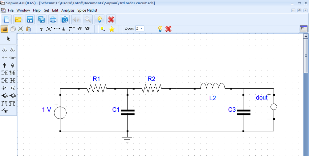
The answer given by periblepsis is very thorough and rigorous but let me just show how Sapwin does the symbolic work quite nicely, through a simple schematic capture interface:

enter image description here

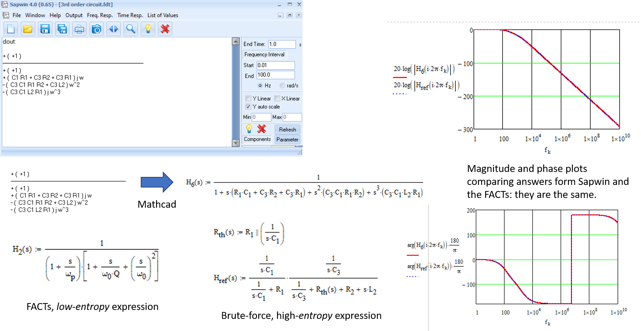
You see a third-order network made of two capacitors and an inductor. I have analyzed this circuit using FACTs some time ago in SE. Here, you capture the circuit by placing the components from the left-side panel and you wire them together as needed. Place the probe dout in the right side which designates the response node. When done, press the star symbol and the symbolic result immediately appears:

enter image description here

I know some of my readers have tested Sapwin on complicated small-signal models - like the PWM switch in a Cuk converter - and the results were correct. A neat free program for those who urgently need a symbolic transfer function.

\$\endgroup\$
2
  • \$\begingroup\$ Thanks for demonstrating this software and making me aware of it! \$\endgroup\$ Commented Sep 21 at 15:52
  • \$\begingroup\$ Avec plaisir ! : ) \$\endgroup\$ Commented Sep 21 at 17:19
2
\$\begingroup\$

Lcapy is a Python library for symbolic linear circuit analysis. Unlike numerical tools like SPICE, it uses SymPy to find analytic expressions such as impedance and transfer functions.

Here are some examples.

2nd Order LC Filter

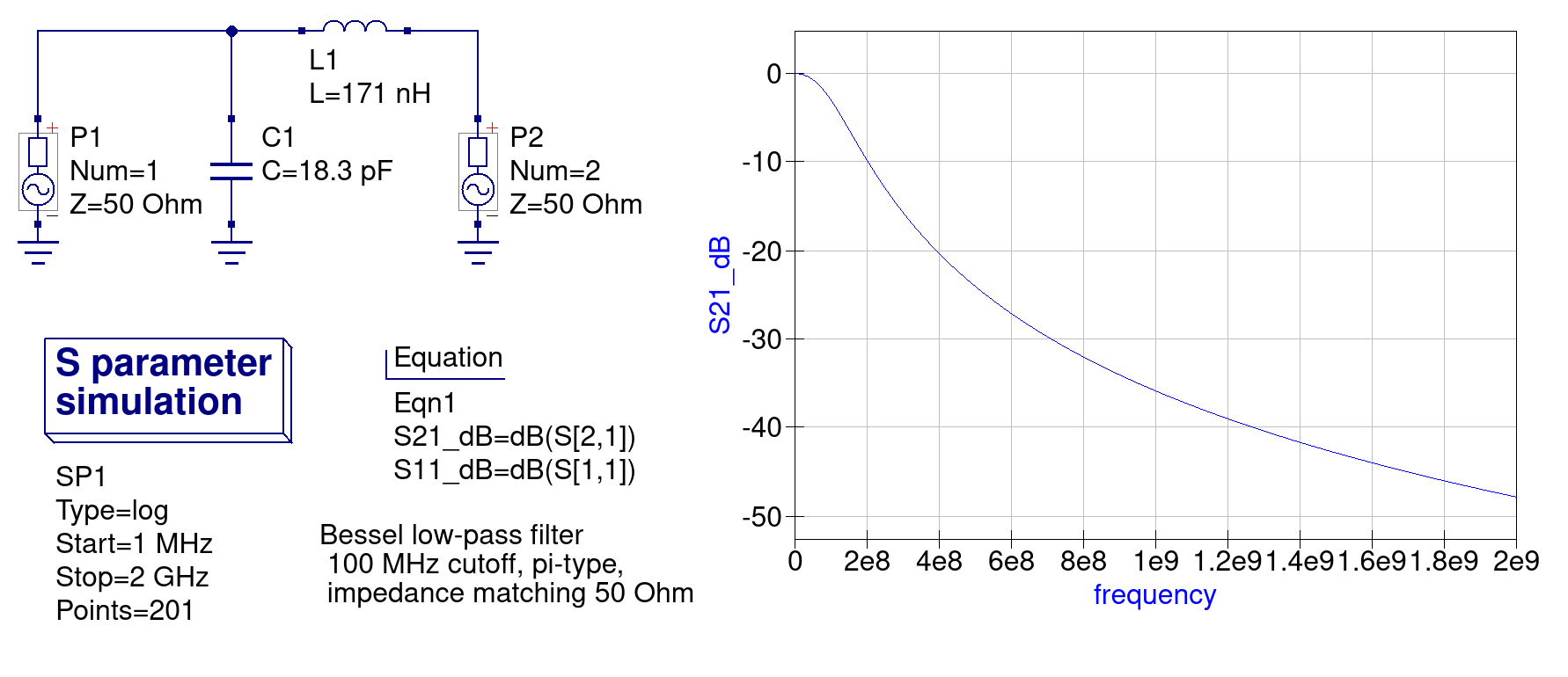
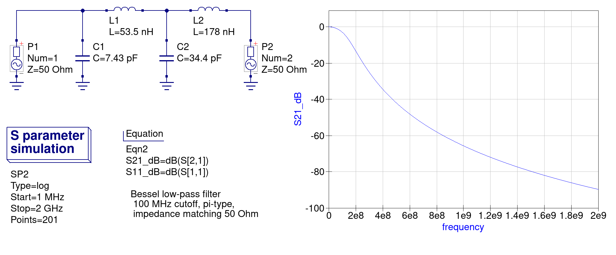
Here's second-order Bessel (LC) low-pass filter with a 100 MHz cutoff, and a roll-off of 40 dB/decade. Its numerical solution is first obtained via Qucs simulator.

A second-order Bessel (LC) filter, and its numerical solution obtained via Qucs simulator.

To find its analytic solution, use the following Lcapy code:

import lcapy 

# define a netlist string
netlist = """
    Rs 1 2
    C1 2 0
    L1 2 3
    Rl 3 0
"""

# create a Circuit object from the netlist
circuit = lcapy.Circuit(netlist)

# Find transfer function between node (0, 1) and (0, 3)
h = circuit.transfer(0, 1, 0, 3).simplify()
print(h)

# Same result, but in TeX
print(circuit.transfer(0, 1, 0, 3).simplify().latex())

The output is:

$$ \frac{R_{l}}{C_{1} L_{1} R_{s} s^{2} + R_{l} + R_{s} + s \left(C_{1} R_{l} R_{s} + L_{1}\right)} $$

To find the time-domain response, perform a reverse Laplace transform:

print(h.inverse_laplace().simplify().latex())

The output is:

$$ \frac{R_{l} \left(e^{\frac{t \sqrt{C_{1}^{2} R_{l}^{2} R_{s}^{2} - 2 C_{1} L_{1} R_{l} R_{s} - 4 C_{1} L_{1} R_{s}^{2} + L_{1}^{2}}}{C_{1} L_{1} R_{s}}} - 1\right) e^{- \frac{t \left(\frac{R_{l}}{L_{1}} + \frac{1}{C_{1} R_{s}} + \frac{\sqrt{C_{1}^{2} R_{l}^{2} R_{s}^{2} - 2 C_{1} L_{1} R_{l} R_{s} - 4 C_{1} L_{1} R_{s}^{2} + L_{1}^{2}}}{C_{1} L_{1} R_{s}}\right)}{2}} u\left(t\right)}{\sqrt{C_{1}^{2} R_{l}^{2} R_{s}^{2} - 2 C_{1} L_{1} R_{l} R_{s} - 4 C_{1} L_{1} R_{s}^{2} + L_{1}^{2}}} $$

Note that analyzing high-order circuit in time domain is strongly discouraged. The resulting machine-generated expression is usually human-unreadable, and no better than a numerical solution. The fact that SymPy is not the most powerful Computer Algebra system certainly doesn't help.

For example, I can manually rewrite the previous result as:

$$ \begin{equation} \left\lbrace \begin{aligned} \tau_1 &= {\frac{\sqrt{C_{1}^{2} R_{l}^{2} R_{s}^{2} - 2 C_{1} L_{1} R_{l} R_{s} - 4 C_{1} L_{1} R_{s}^{2} + L_{1}^{2}}}{C_{1} L_{1} R_{s}}} \\ \tau_2 &= {- \frac{\left(\frac{R_{l}}{L_{1}} + \frac{1}{C_{1} R_{s}} + \frac{\sqrt{C_{1}^{2} R_{l}^{2} R_{s}^{2} - 2 C_{1} L_{1} R_{l} R_{s} - 4 C_{1} L_{1} R_{s}^{2} + L_{1}^{2}}}{C_{1} L_{1} R_{s}}\right)}{2}} \\ h(t) &= u(t) \dfrac{R_{l} \left(e^{\tau_1 t} - 1\right) (e^{\tau_2 t})}{\sqrt{C_{1}^{2} R_{l}^{2} R_{s}^{2} - 2 C_{1} L_{1} R_{l} R_{s} - 4 C_{1} L_{1} R_{s}^{2} + L_{1}^{2}}} \end{aligned} \right. \end{equation} $$

For second-order systems, the expressions is barely readable. For higher-order systems. For 3rd-order and high-order systems it's unmanageable. Furthermore, Lcapy takes almost forever (many hours) to generate and simplify a solution, as it's not optimized to handle these tasks.

Thus, use the proper tool for the job, and stay in the frequency domain or S domain.

3nd Order LC Filter

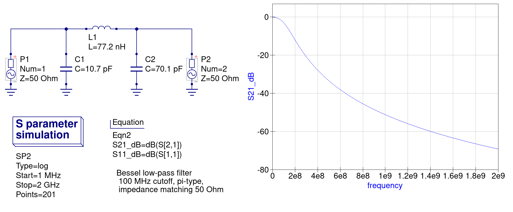
As another example, here is a third-order Bessel (LC) low-pass filter with a 100 MHz cutoff, and a roll-off of 60 dB/decade. Its numerical solution is first obtained via Qucs simulator.

A 3rd Order Bessel filter and its numerical solution in Qucs

To find its analytic solution:

import lcapy 

netlist = """
    Rs 1 2
    C1 2 0
    L1 2 3
    C2 3 0
    Rl 3 0
"""

circuit = lcapy.Circuit(netlist)
h = circuit.transfer(0, 1, 0, 3).simplify()
print(h.latex())

# Warning: This calculation takes half an hour on a high-end
# CPU core with a thousand-character output. If `simplify()`
# is used, SymPy is never designed for big problems, so its
# limited performance means it probably won't terminate before
# the heat death of the universe.
print(h.inverse_laplace())

The analytic transfer function obtained by Lcapy is:

$$ \dfrac{R_{l}}{C_{1} C_{2} L_{1} R_{l} R_{s} s^{3} + L_{1} s^{2} \left(C_{1} R_{s} + C_{2} R_{l}\right) + R_{l} + R_{s} + s \left(C_{1} R_{l} R_{s} + C_{2} R_{l} R_{s} + L_{1}\right)} $$

4nd Order LC Filter

As another example, here is a fourth-order Bessel (LC) low-pass filter with a 100 MHz cutoff, and a roll-off of 80 dB/decade. Its numerical solution is first obtained via Qucs simulator.

A 4rd Order Bessel filter and its numerical solution in Qucs

We can ask Lcapy to find its transfer function with the following code:

import lcapy 

netlist = """
    Rs 1 2
    C1 2 0
    L1 2 3
    C2 3 0
    L2 3 4
    Rl 4 0
"""

circuit = lcapy.Circuit(netlist)
h = circuit.transfer(0, 1, 0, 4).simplify()
print(h.latex())

The output is:

$$ \dfrac{R_{l}}{C_{1} C_{2} L_{1} L_{2} R_{s} s^{4} + C_{1} C_{2} L_{1} R_{l} R_{s} s^{3} + C_{1} L_{1} R_{s} s^{2} + C_{1} L_{2} R_{s} s^{2} + C_{1} R_{l} R_{s} s + C_{2} L_{1} L_{2} s^{3} + C_{2} L_{1} R_{l} s^{2} + C_{2} L_{2} R_{s} s^{2} + C_{2} R_{l} R_{s} s + L_{1} s + L_{2} s + R_{l} + R_{s}} $$

8-Resistor Bridge

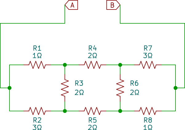
And now for something completely different: Let's try the following 8-resistor bridge circuit, we want to find the impedance between node A and B.

An 8-resistor bridge

This was the subject of as an earlier question Can we find the equivalent resistance just by using series and parallel combinations?. Under that question, I've showed that by using Extra Element Theorem (EET) - a lesser known circuit analysis technique, original invented by professor R. D. Middlebrook at Caltech - it was possible to derive its complicated analytic solution while keeping the size of equations under control, making it possible to do the derivation by hand without a computer.

To show that the result obtained by EET was valid, I used Lcapy to generate a mechanical analytic solution:

from lcapy import Circuit

circuit = ("""
    R1 1 2
    R2 3 4
    R3 2 4
    R4 2 5
    R5 4 6
    R6 5 6
    R7 5 7
    R8 6 8
    W1 7 8
    W2 1 3
    W3 1 9
    W4 7 10
    P1 9 10
""")

print(str(circuit.impedance("P1")))

The output is:

(R1*R2*R3*R6 + R1*R2*R3*R7 + R1*R2*R3*R8 + R1*R2*R4*R6 + R1*R2*R4*R7 + R1*R2*R
4*R8 + R1*R2*R5*R6 + R1*R2*R5*R7 + R1*R2*R5*R8 + R1*R2*R6*R7 + R1*R2*R6*R8 + R
1*R3*R5*R6 + R1*R3*R5*R7 + R1*R3*R5*R8 + R1*R3*R6*R8 + R1*R3*R7*R8 + R1*R4*R5*
R6 + R1*R4*R5*R7 + R1*R4*R5*R8 + R1*R4*R6*R8 + R1*R4*R7*R8 + R1*R5*R6*R7 + R1*
R5*R7*R8 + R1*R6*R7*R8 + R2*R3*R4*R6 + R2*R3*R4*R7 + R2*R3*R4*R8 + R2*R3*R6*R7
 + R2*R3*R7*R8 + R2*R4*R5*R6 + R2*R4*R5*R7 + R2*R4*R5*R8 + R2*R4*R6*R8 + R2*R4
*R7*R8 + R2*R5*R6*R7 + R2*R5*R7*R8 + R2*R6*R7*R8 + R3*R4*R5*R6 + R3*R4*R5*R7 +
 R3*R4*R5*R8 + R3*R4*R6*R8 + R3*R4*R7*R8 + R3*R5*R6*R7 + R3*R5*R7*R8 + R3*R6*R
7*R8)/(R1*R3*R6 + R1*R3*R7 + R1*R3*R8 + R1*R4*R6 + R1*R4*R7 + R1*R4*R8 + R1*R5
*R6 + R1*R5*R7 + R1*R5*R8 + R1*R6*R7 + R1*R6*R8 + R2*R3*R6 + R2*R3*R7 + R2*R3*
R8 + R2*R4*R6 + R2*R4*R7 + R2*R4*R8 + R2*R5*R6 + R2*R5*R7 + R2*R5*R8 + R2*R6*R
7 + R2*R6*R8 + R3*R4*R6 + R3*R4*R7 + R3*R4*R8 + R3*R5*R6 + R3*R5*R7 + R3*R5*R8
 + R3*R6*R7 + R3*R6*R8)

After simplification, in TeX:

$$ \frac{{\left(R_{1} R_{2} R_{3} + {\left(R_{1} R_{2} + R_{2} R_{3}\right)} R_{4} + {\left(R_{1} R_{2} + R_{1} R_{3} + {\left(R_{1} + R_{2} + R_{3}\right)} R_{4}\right)} R_{5}\right)} R_{6} + {\left(R_{1} R_{2} R_{3} + {\left(R_{1} R_{2} + R_{2} R_{3}\right)} R_{4} + {\left(R_{1} R_{2} + R_{1} R_{3} + {\left(R_{1} + R_{2} + R_{3}\right)} R_{4}\right)} R_{5} + {\left(R_{1} R_{2} + R_{2} R_{3} + {\left(R_{1} + R_{2} + R_{3}\right)} R_{5}\right)} R_{6}\right)} R_{7} + {\left(R_{1} R_{2} R_{3} + {\left(R_{1} R_{2} + R_{2} R_{3}\right)} R_{4} + {\left(R_{1} R_{2} + R_{1} R_{3} + {\left(R_{1} + R_{2} + R_{3}\right)} R_{4}\right)} R_{5} + {\left(R_{1} R_{2} + R_{1} R_{3} + {\left(R_{1} + R_{2} + R_{3}\right)} R_{4}\right)} R_{6} + {\left({\left(R_{1} + R_{2}\right)} R_{3} + {\left(R_{1} + R_{2} + R_{3}\right)} R_{4} + {\left(R_{1} + R_{2} + R_{3}\right)} R_{5} + {\left(R_{1} + R_{2} + R_{3}\right)} R_{6}\right)} R_{7}\right)} R_{8}}{{\left({\left(R_{1} + R_{2}\right)} R_{3} + {\left(R_{1} + R_{2} + R_{3}\right)} R_{4} + {\left(R_{1} + R_{2} + R_{3}\right)} R_{5}\right)} R_{6} + {\left({\left(R_{1} + R_{2}\right)} R_{3} + {\left(R_{1} + R_{2} + R_{3}\right)} R_{4} + {\left(R_{1} + R_{2} + R_{3}\right)} R_{5} + {\left(R_{1} + R_{2} + R_{3}\right)} R_{6}\right)} R_{7} + {\left({\left(R_{1} + R_{2}\right)} R_{3} + {\left(R_{1} + R_{2} + R_{3}\right)} R_{4} + {\left(R_{1} + R_{2} + R_{3}\right)} R_{5} + {\left(R_{1} + R_{2} + R_{3}\right)} R_{6}\right)} R_{8}} $$

This solution was then compared with the hand solution via SageMath to show its validity. Check the original question for more details.

\$\endgroup\$

Your Answer

By clicking “Post Your Answer”, you agree to our terms of service and acknowledge you have read our privacy policy.

Not the answer you're looking for? Browse other questions tagged or ask your own question.