Ebers-Moll Model
$$
\begin{align}
I_{\mathrm{b}} & = \frac{I_{\mathrm{s}}}{\beta_{\mathrm{f}}}\left(\mathrm{e}^{\frac{V_{\mathrm{eb}}}{NV_{\mathrm{t}}}} - 1\right) + \frac{I_{\mathrm{s}}}{\beta_{\mathrm{r}}}\left(\mathrm{e}^{\frac{V_{\mathrm{eb}} - V_{\mathrm{ec}}}{NV_{\mathrm{t}}}} - 1\right)
\\[0.9em]
I_{\mathrm{c}} &= I_{\mathrm{s}}\left(\mathrm{e}^{\frac{V_{\mathrm{eb}}}{NV_{\mathrm{t}}}} - 1\right) - I_{\mathrm{s}}\frac{\beta_{\mathrm{r}} + 1}{\beta_{\mathrm{r}}}\left(\mathrm{e}^{\frac{V_{\mathrm{eb}} - V_{\mathrm{ec}}}{NV_{\mathrm{t}}}} - 1\right).
\end{align}
$$
Model parameters:
- Saturation current \$I_\mathrm{s}\$
- Ideality factor \$N\$
- Thermal voltage \$V_\mathrm{t}\$
- Forward gain \$\beta_\mathrm{f}\$
- Reverse gain \$\beta_\mathrm{r}\$
Direct parameter extraction
The most straight-forward way of finding parameter values for the Ebers-Moll model from measurements is using direct extraction.
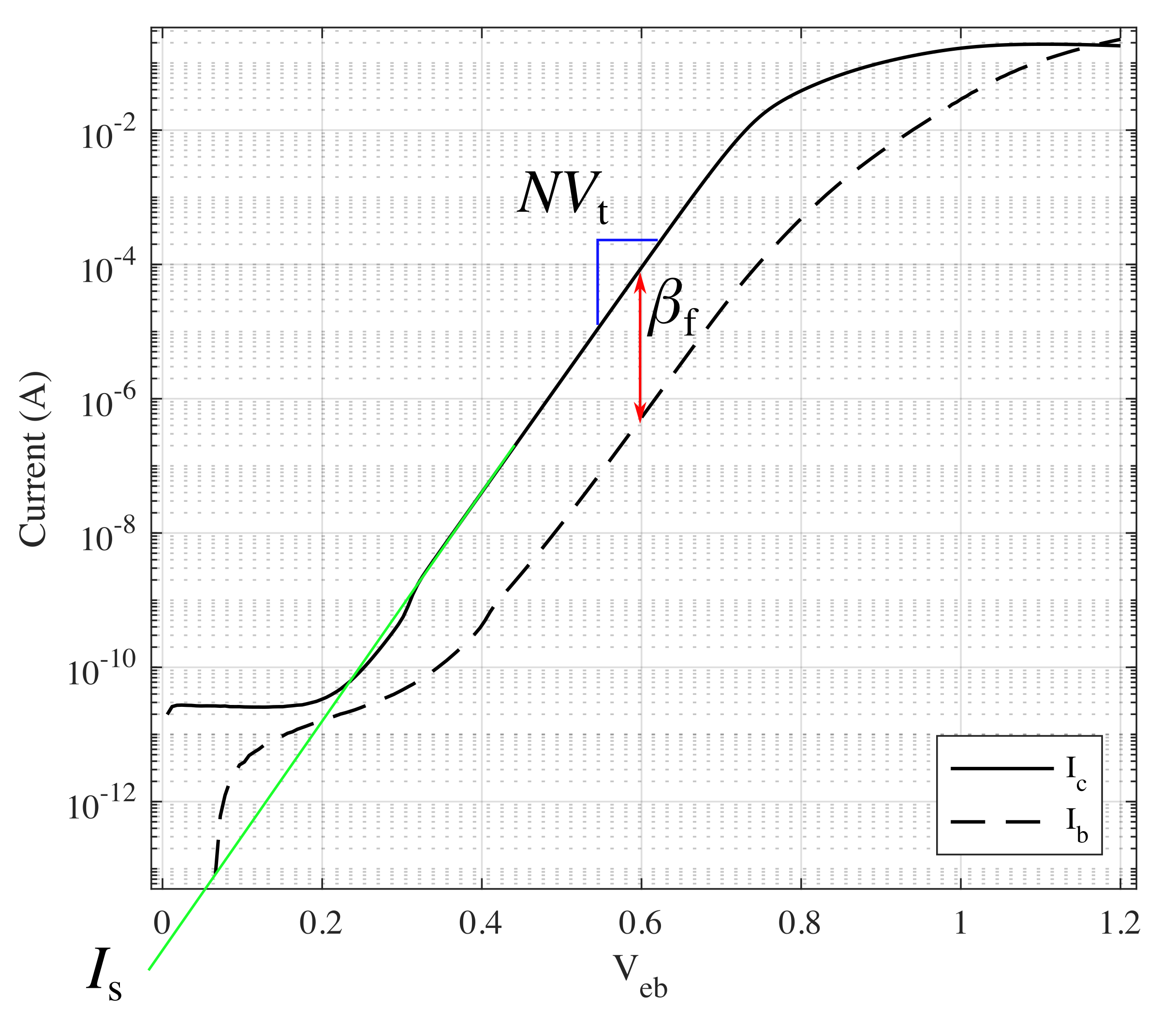
The below figure illustrates a Forward Gummel measurement of the 2N3906 BJT, which is when \$V_\mathrm{ec}\$ is kept a constant potential and \$V_\mathrm{eb}\$ is swept over a range. For this figure \$V_\mathrm{ec} = 0.3\ \text{V}\$. (As an aside I chose this badly as you want the value of \$V_\mathrm{eb} - V_\mathrm{ec}\$ to be small for the Ebers-Moll model to be a good approximation).

In the middle of the measurement we see an ideal region which appears linear but is actually exponential as the current is on a logarithmic axis. The Ebers-Moll model only captures the exponential behaviour of the BJT and not the high and low-current regions, so the parts at the top and bottom can be ignored. From the middle of the measurement 3 out of 4 parameters can be determined.
The gradient of the ideal region controlled by the parameter combination \$ N V_\mathrm{t} \$. Inspecting the Ebers-Moll equations when biased in the forward-active region (i.e. \$V_\mathrm{eb} - V_\mathrm{ec}\$ is negative) we can see
$$
I_\mathrm{c} = I_\mathrm{s} \mathrm{e}^\frac{V_\mathrm{eb}}{NV_\mathrm{t}}
$$
where \$NV_\mathrm{t}\$ is the gradient of the exponential current with respect to \$V_\mathrm{eb}\$. The thermal voltage can be found by measuring the junction temperature during the current measurements and applying this formula.
Also from this equation we can see that when the exponent is 0, \$I_\mathrm{c} = I_\mathrm{s}\$. When \$V_\mathrm{eb}\$ approaches 0 however the BJT does not behave ideally, so to find \$I_\mathrm{s}\$ we extrapolate from the ideal region.
Finally the gain can be found from the approximation \$I_\mathrm{c} = I_\mathrm{b}\beta_\mathrm{f}\$, i.e. by selecting a point in the ideal region and finding the multiplicative difference.
For reverse measurements \$V_\mathrm{eb}\$ is simply made negative which reveals a similar plot but with the reverse gain factor \$\beta_\mathrm{r}\$.
References
Ian Getreu, 'Modeling the Bipolar Transistor', 1976, Tektronix

