How do you plot pulse positions for a simple sine wave in MATLAB?

Question

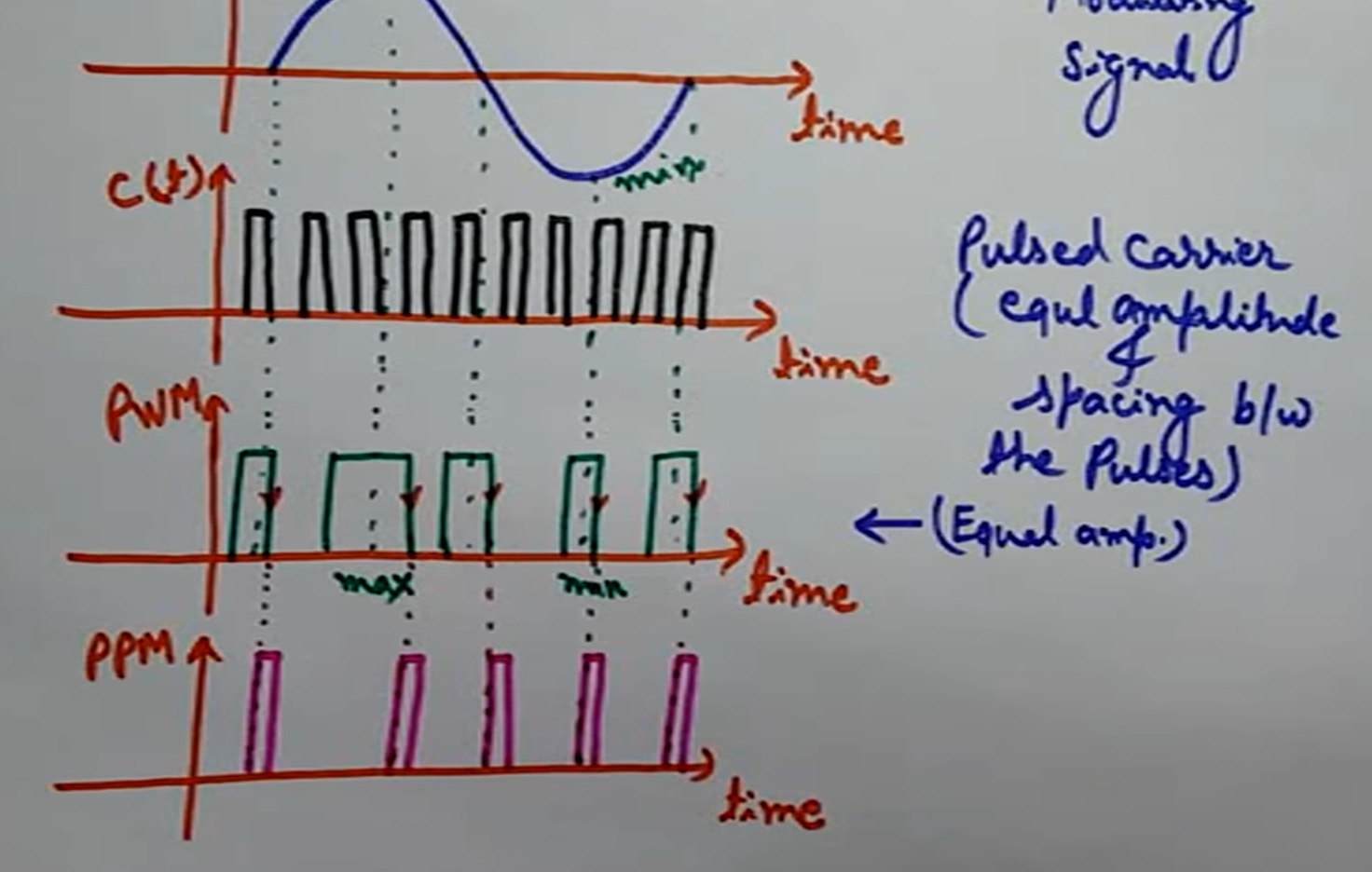
If you goto 14 minutes and 53 seconds of this video: https://youtu.be/xfxQ-zBp2OQ you will see a plot of Pulse Width Modulation (PWM) and Pulse Position Modulation (PPM) for a simple sine wave signal.

The picture should look something like this:

How do I implement a PPM for a sine wave in MATLAB? Here is what I am thinking:

t = 0:1/1e3:60;
d = [0:2:60;sin(2*pi*0.05*(0:2:60))]';
x = @rectpuls;
y = pulstran(t,d,x);
plot(t,y)
hold off
xlabel('Time (s)')
ylabel('Waveform')

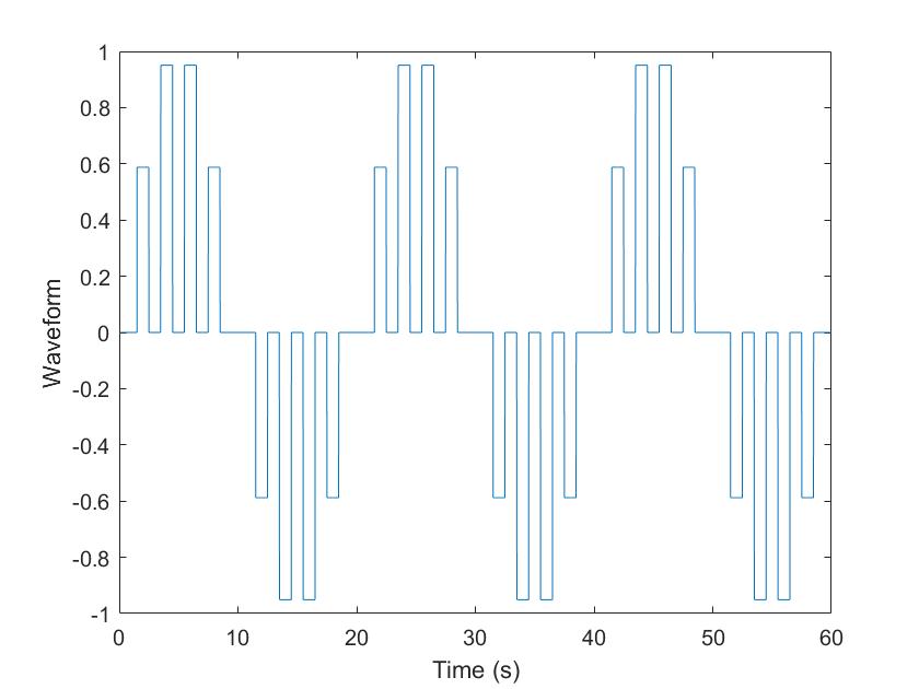
But this gives me a plot of rectangular samples of the sine wave:

not the PPM as shown in the first graphic above.

So even though I understand what the YouTuber is doing graphically, I'm not sure how this can be implemented in MATLAB from an algorithmic standpoint.

I would appreciate any feedback from the EE community.

Answer 1

It turns out this code does exactly what I want:

code sample 8 from: https://www.jcbrolabs.org/matlab-codes

% This file simulate Pulse Position Modulation (PPM) as per message signal amplitude
% 
% Created By: JCBRO Labs
% Date: 03/06/2017
% website: www.jcbrolabs.org
% mail: [email protected]
clc; clear all; close all;
fc = 20;    %carrier frequency
fm = 2;     % message frequency
fs = 1000;  % sampling frequency
t = 1;  
n = [0:1/fs:t];
n = n(1:end - 1);
duty = 10;
% no. of samples in one square wave period
per = fs/fc;
% no. of samples in on time
on_t = per/duty;

s = square(2*pi*fc*n,duty);
s(find(s<0)) = 0;
% message signal
m = sin(2*pi*fm*n);

% Triangular wave
A=1.25;
c=A.*sawtooth(2*pi*fc*n);%Carrier sawtooth

% 
ppm = zeros(1,length(s));

% find ids where carrier is greater than message
id = find(c > m);
idd = diff(id);
iddd = find(idd ~= 1);
temp(1) = id(1);
temp(2:length(iddd)+1) = id(iddd + 1);

% ppm signal
for i = 1:length(temp)
    ppm(temp(i) : temp(i) + on_t - 1) = 1;
end
% Plot
subplot(3,1,1);plot(n,m,'LineWidth',2);title('Message Signal');hold on; plot(n,c,'r','LineWidth',2);grid on;
subplot(3,1,2);plot(n,s,'LineWidth',2);title('Pulse Train');grid on; ylim([-0.2 1.2]);
subplot(3,1,3);plot(n,ppm,'LineWidth',2);title('PPM Signal'); grid on; ylim([-0.2 1.2]);

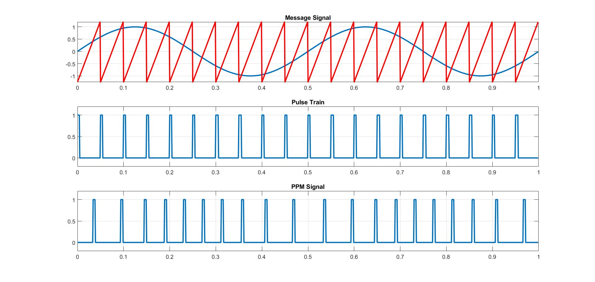
Running this code gives: