I am asking what is the difference between time-domain frequency analysis and “normal” frequency analysis in LTspice?
LTspice is nothing but a SPICE solver, so .AC, or .TRAN, are the same as in every other SPICE program, with the sole differences being in the way the solvers, themselves, are implemented under the hood.
An .AC analysis relies on solving the circuit for an operating point, after which it is solved considering its response to a small signal, using complex values.
If the circuit is linear (e.g. RLC) then it does not need any special considerents -- the inductances are shorted, the capacitances opened, and the whole circuit is treated as a resistive network, which gives its operating point. Any small signal analysis is known to be accurate since the circuit will respond the same whether the input signal is 1 mV or 1 kV.
But if the circuit is nonlinear (e.g. a diode) then the analysis is done on a small slope around the operating point, because having a larger signal would cause nonlinear distortions.

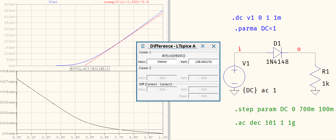
To give an example, in the top graph, the blue trace shows the characteristic curve of a 1N4148. The red trace is (a hammered) slope representing the slope for the operating point at 700 mV. The small signal is approximated to be ~1 mV, because it is considered that its amplitude will, largely, not be affected by the nonlinearity of the system. That is, around the operating point, the characteristic curve can be considered a slope -- linear.
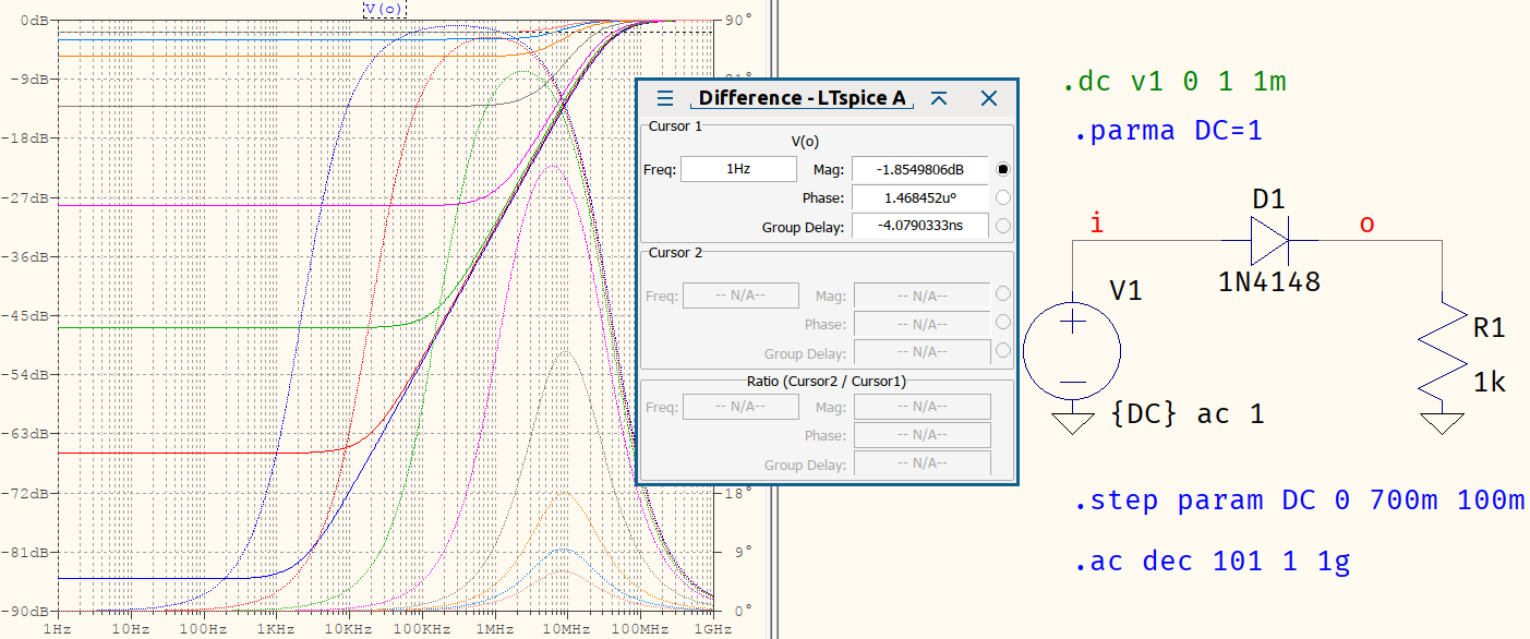
The dynamic resistance of the diode is plotted at the bottom, and the value at 700 mV is shown to be 238.06 Ω. Now, if you were to perform an .AC analysis for the same circuit, while using various DC levels for the source (from 0 to 700 mV, in 100 mV increments), you would get this graph:

Notice that the output is not flat and also varies with the different levels of polarization. And, using the cursors to measure the value at 1 Hz (.AC can't use DC) you see -1.85498 dB, which is:
$$20\log_{10}\left(\dfrac{1000}{1000+238.06317}\right)=-1.854856$$
Which is close enough given the truncation. This is why the .AC is called the small signal analysis: everything revolves around a small region on the operating point. Also, that operating point is considered to be the steady-state of the system.
A .TRAN analysis is done using real numbers and it may, or may not involve an operating point. This is because the signals can have any amplitude, so that the transient (.TRAN) effects can be studied in time domain. While you can perform an .AC in .TRAN, it is prone to numeric precision due to the limited numeric precision of the .raw file (by default it's in float; it needs .opt numdgt=7 to be double) and that of the waveform compression (can be disabled with .opt plotwinsize=0). It's also polluted with nonlinearities, since it's highly unlikely that the analysis will be done with small levels, 1 mV or below. Not lastly, it is tedious, because not only you need to run a frequency-swept signal, you need to wait for all the transients to die out so that you are in the steady-state, and detecting that is, again, affected by the limited numerical precision that .TRAN uses.
This is why .TRAN is known as the large signal analysis.
With these in mind, ...
When can you use which one?
If you are interested in the small signal frequency response of the system -- that is, you know that the system is, or is very close to being linear for the given signals, then .AC is for you. As per @The Photon's remark, you also have to consider that the system allows a frequency analysis (in LTspice, SMPSs can be analyzed, but it's not perfect; also see the rest of the answers in there).
If you are interested in the time domain response, that is, you want to see the nitty-gritty details of the transitory moments before the system settles, or how the signals are distorted (or not), then .TRAN is for you.
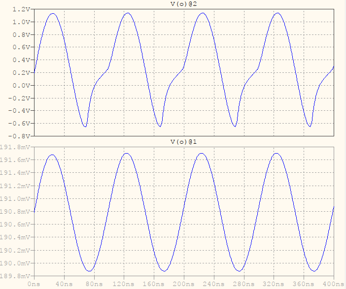
To use the same circuit as above, in .AC you get the graphs above, but in .TRAN, with the same 700 mV offset, a 10 MHz will yield one thing with a sine of 1 mV amplitude (bottom trace) versus 1 V amplitude (top):

If you do the math, for the 1 mV amplitude, 700 mV offset case, the output to input ratio can be calculated with these lines:
.meas avgo avg v(o)               ; output offset
.meas rmso rms v(o)-avgo          ; RMS without offset
.meas mag param rmso/(1m/sqrt(2)) ; magnitude of output/input
.meas db param 20*log10(mag)      ; dB(magnitude)
.meas to when v(o)-avgo=0 fall=4  ; "zero" crossing for output
.meas ti when v(i)-0.7=0 fall=4   ; "zero" crossing for input
.meas rad param (ti-to)/0.1u*2*pi ; phase difference, radians
.meas deg param rad*180/pi        ; phase difference, degrees
The 1m/sqrt(2) is the RMS of the input, withou the DC. The results are:
avgo: AVG(v(o))=0.190784 FROM 0 TO 4e-007
rmso: RMS(v(o)-avgo)=0.000644485 FROM 0 TO 4e-007
mag: rmso/(1m/sqrt(2))=0.911439
db: 20*log10(mag)=-0.805444
to: v(o)-avgo=0 AT 3.48408e-007
ti: v(i)-0.7=0 AT 3.5e-007
rad: (ti-to)/0.1u*2*pi=0.100024
deg: rad*180/pi=5.73095
If you run an .AC at one single frequency, 10 MHz, as the signal, you get:
V(o): mag: 0.915904 phase: 5.99033°
0.911439 ~ 0.915904 and 5.73095 ~ 5.99033, which is quite close. The same analysis is no longer possible for the 1 V amplitude -- that would be the large signal response and it involves nonlinearities.
Nonlinear distortions are .TRAN's speciality, frequency responses are .AC's.

