1
\$\begingroup\$

I have the following (badly formulated) problem.

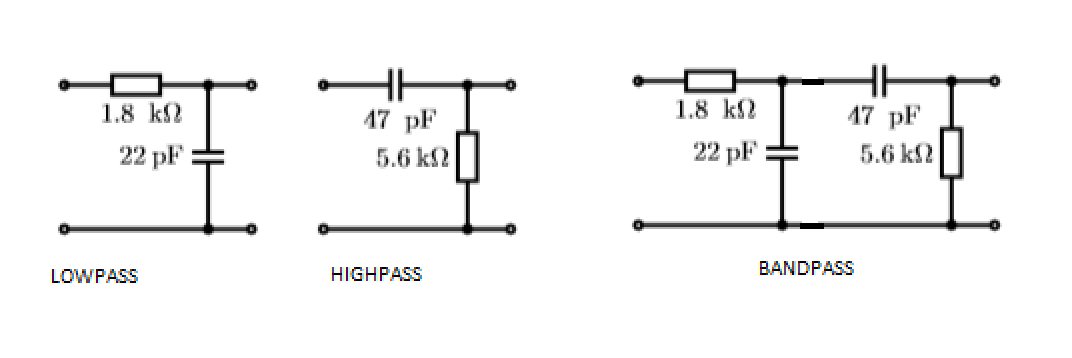
A passive first order lowpass filter gets cascaded with a passive first order highpass filter to form a bandpass as the following circuit diagram shows.

enter image description here

By how many percent does the lowpass behavior (upper pole frequency) of the resulting filter move with respect to the frequency of the pole of the original lowpass filter?

I tried to solve this problem using LT-spice, because I couldn't find a way to solve it algebraically.

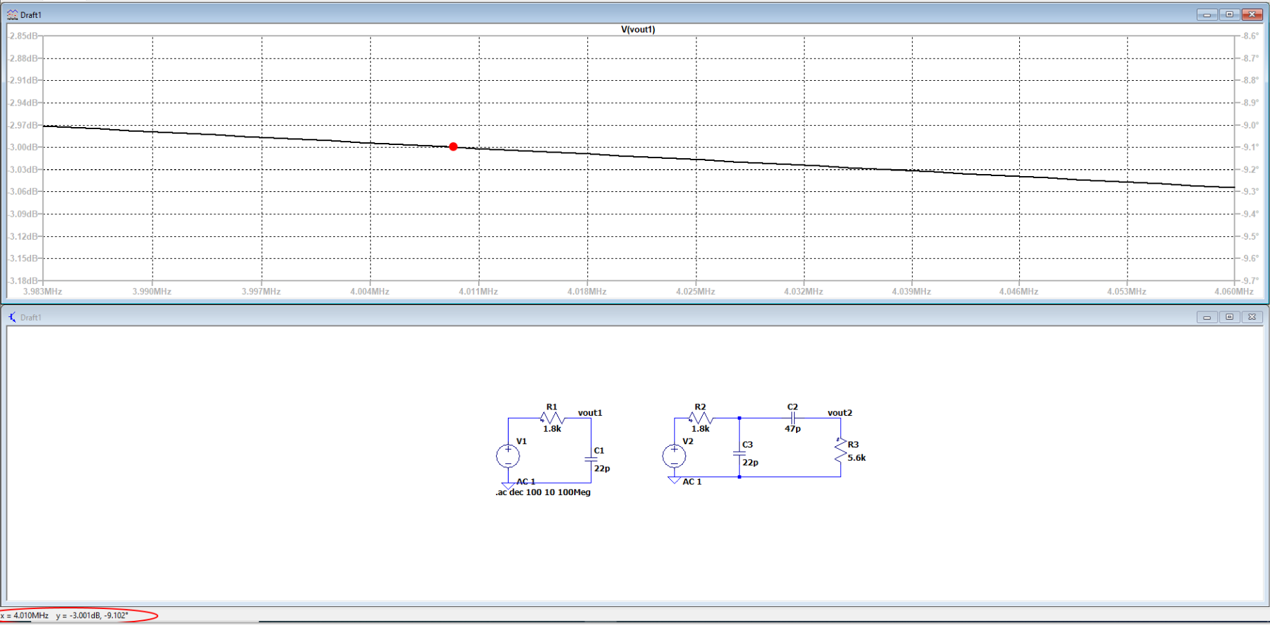
Here is the lowpass filter simulated. I found the -3db gain to be at \$f=4.10\$MHz. And that must mean that the pole for this filter is at 4.10MHz, right?

enter image description here

I also tried to simulate the bandpass filter, but it turns out that it never reaches -3db gain.

So if I can't find the pole for the bandpass filter, I can't solve the problem. I hope someone can help me with this, either algebraically and or with LT-spice.

EDIT

Trying to solve this problem algebraically with a lot of help from VerbalKint.

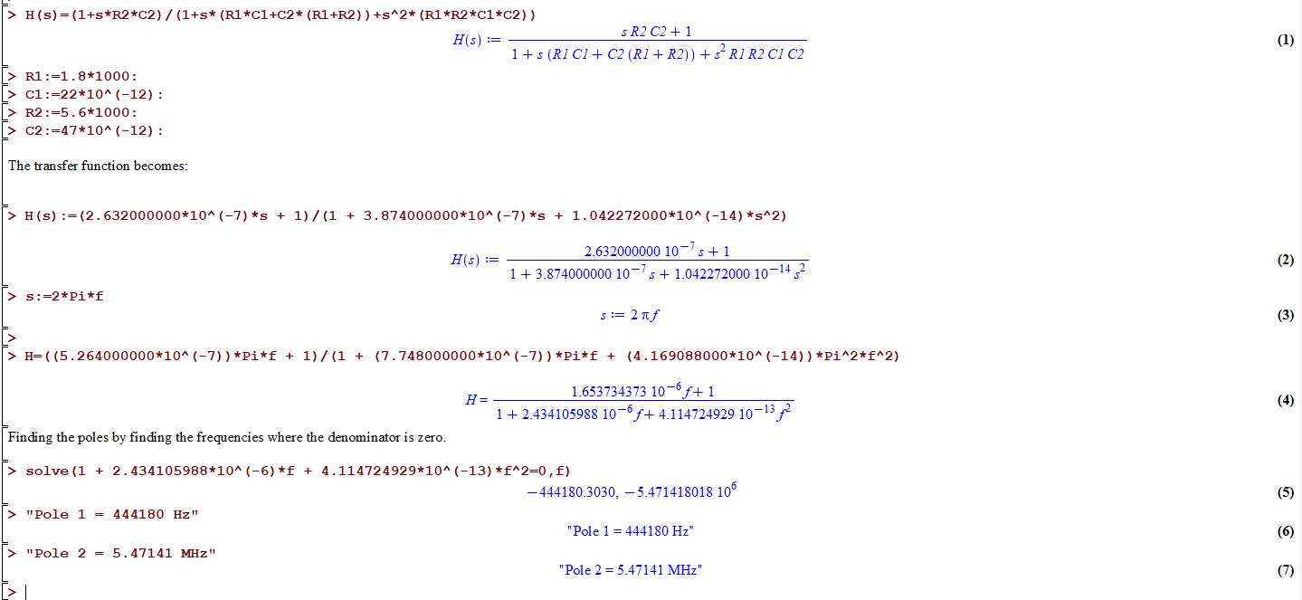
Using the transfer function he provided, I tried to solve this with Maple.

enter image description here

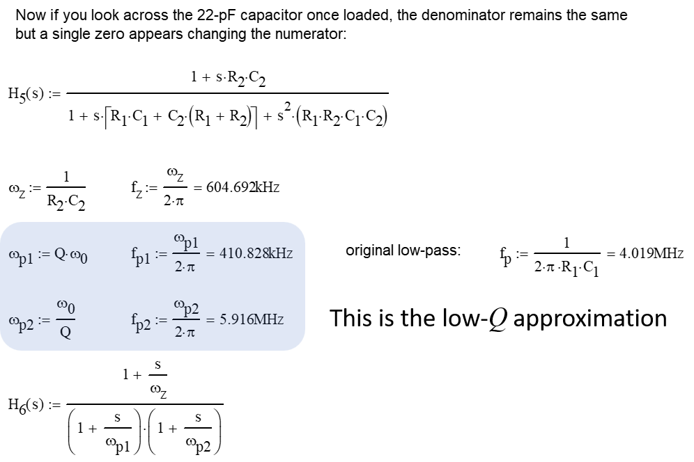
As you can see I get the pole frequencies to be at: \$f=444180 \text{MHz} \$ and \$f=5.47141 \text{MHz} \$.

These frequencies are very close to what VerbalKint provided, but there is still a difference. I wonder what have gone wrong in my calculations.

\$\endgroup\$
11
  • 2
    \$\begingroup\$ Hint: if you place the two sections right one after another, the "loading effect" happens (the next stage influences the previous one). If you add a buffer, you will avoid that. However, this is a problem that can be solved on paper. \$\endgroup\$ Commented Apr 14, 2020 at 20:26
  • 1
    \$\begingroup\$ @VerbalKint Look right below OP's 1st picture. That's why I suggested the buffer, for easier measuring. I also said this could have been done on paper. It's OP's choice. \$\endgroup\$ Commented Apr 14, 2020 at 21:01
  • 1
    \$\begingroup\$ @Carl Don't forget to also check the bandwidth of that opamp. Better yet, use a VCVS (E-source) for that. \$\endgroup\$ Commented Apr 14, 2020 at 21:02
  • 1
    \$\begingroup\$ @a concerned citizen, well the text says how many percent does the low-pass behavior changes once loaded so I assume this is the entire network that needs consideration and not with the insertion of the buffer. Otherwise it's too easy : ) \$\endgroup\$ Commented Apr 14, 2020 at 21:05
  • 1
    \$\begingroup\$ @VerbalKint No doubt, but since OP preferred a simulator over the pen and paper... be careful what you wish for. :-) \$\endgroup\$ Commented Apr 14, 2020 at 21:08

1 Answer 1

2
\$\begingroup\$

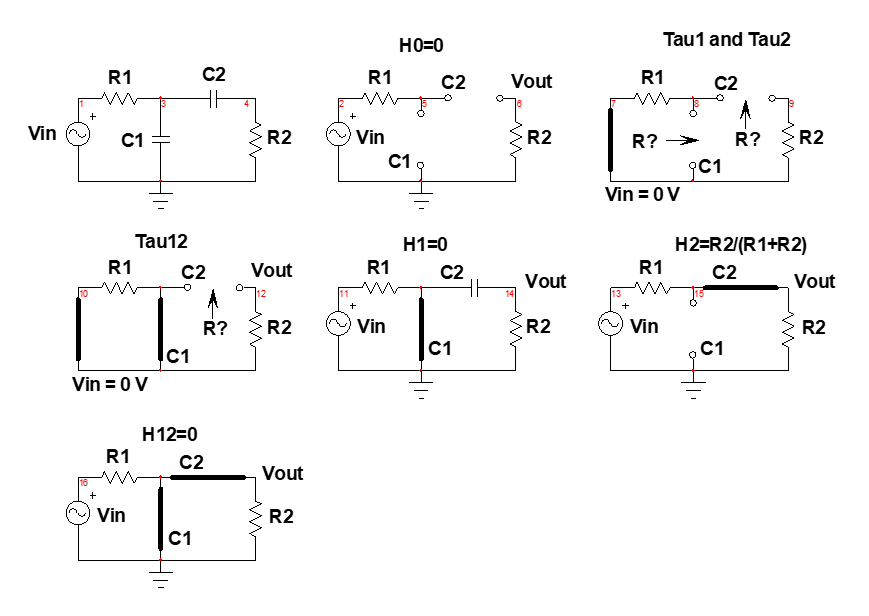
The transfer function of these cascaded filters can be determined using the fast analytical circuits techniques or FACTs. You need to determine the time constants involving the energy-storing elements when the stimulus is zeroed. To do so, temporarily disconnect the capacitors and "look" through their connecting terminals to determine the resistance \$R\$ you want to determine the time constant:

enter image description here

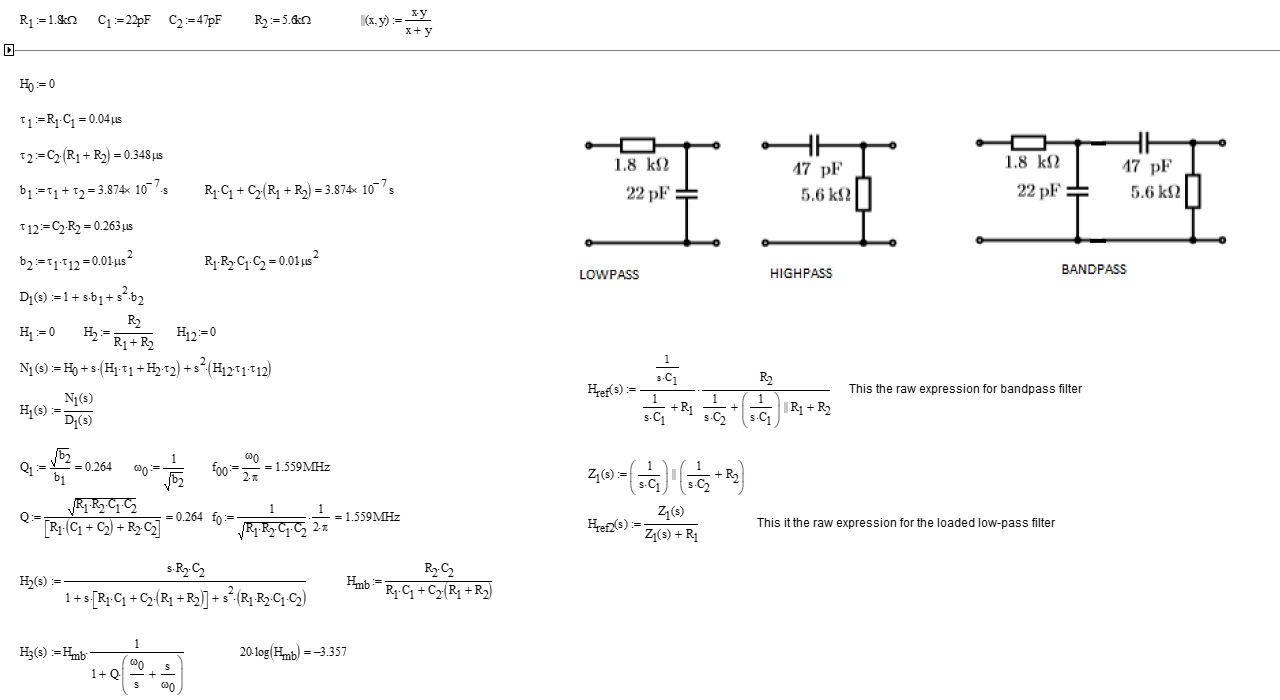
Once there, you find the gains \$H\$ of this circuit when all caps are open-circuited (\$s=0\$) and then when they alternatively shorted. You do it without writing a line of algebra, just by inspecting the circuit. This is the cool thing about FACTs. Once you have these gains (only 1 is non-zero), then Mathcad does the rest : )

enter image description here

And the resulting plot is that of a band-pass filter centered at 1.6 MHz. Please note that the transfer function \$H_3(s)\$ is expressed in a low-entropy way, showing the band-pass gain or attenuation:

enter image description here

Now, if you want to probe the voltage across \$C_1\$ once loaded by the second filter, the time constants do not change and you can keep the denominator you have already determined. A zero is still there but it no longer occurs at the origin:

enter image description here

By loading the low-pass filter, you actually create a second pole whose position can be determined using the low-\$Q\$ approximation. The below plot shows you the final result if you probe the output voltage across the 22-pF capacitor once loaded:

enter image description here

You can learn more about these FACTs by looking at the book I published on the subject but also reading the APEC seminar I taught in 2016.

\$\endgroup\$
5
  • \$\begingroup\$ Wow! This is just amazing! I really appreciate you helping me with this stuff. And you keep mentioning these FACTS that can let you arrive at the transfer function. Now I am going to study them a bit, cause they seem very useful! \$\endgroup\$
    – Carl
    Commented Apr 14, 2020 at 21:29
  • \$\begingroup\$ oh it is. Via @verbalKint here and C.Basso in re-learning PSU's I came across the concept. It takes a bit to essentially break old habits but it is extremely useful. I have recently followed the steps to analyse an EMI filter but stopped at 3rd order... I need a bit more time to figure out how to incorporate the LISN but thats 6th order and a bit too much for me at the moment, too many permutations as you collect the time constants and I am not fully fluid in the steps \$\endgroup\$
    – user16222
    Commented Apr 15, 2020 at 0:55
  • \$\begingroup\$ Thank you for the laudatory comments. When you've tasted the FACTs, there is no coming back : ) What is nice then is that you "see" where the poles and zeroes are located by looking up a schematic and this is extremely rewarding once you've acquired the skill. For those interested, I have published a 6th-order analysis showing how to collect the terms. Again, you break the circuit into a succession of small sketches that you individually solve: care and time are all it takes ^_^ \$\endgroup\$ Commented Apr 15, 2020 at 6:39
  • \$\begingroup\$ @VerbalKint one last question. The "low-Q approximation", is it precise enough to give a spot on correct result, or is it just an "approximation" ´with some inacurracies? \$\endgroup\$
    – Carl
    Commented Apr 15, 2020 at 7:26
  • 1
    \$\begingroup\$ In a 2nd-order network, the poles split for a quality factor \$Q\$ below 0.5 and become real. Usually, the approximation works for low values of \$Q\$. You do not look for a perfect match between the approximated polynomial but more a formula with a practical usage in determining a component value. You thus accept a small error between what you obtain with the approximation and what the full-blown - probably difficult to use - expression would give. See this document for a comprehensive study of the subject \$\endgroup\$ Commented Apr 15, 2020 at 8:09

Your Answer

By clicking “Post Your Answer”, you agree to our terms of service and acknowledge you have read our privacy policy.

Not the answer you're looking for? Browse other questions tagged or ask your own question.