Qucs simulation of quarter wave microstrip stub doesn't match ideal calculaton

Question

I'm trying to simulate the resonant frequency and insertion loss of a 3 mm open stub on a 10 mm microstrip transmission line (50 Ω) on a FR-4 PCB (εr = 4.0, height = 0.1 mm). I calculated that the microstrip width should be around 0.188 mm.

Ideally, it should resonate and produce a deep null in the insertion loss graph, exactly at 1/4 wavelength, which is \$ f = \frac{v}{4l} \$. And ideally, the speed of light is \$ \frac{c}{\sqrt{\epsilon_r}} \$, so it's \$ f = \frac{c}{4l\sqrt{\epsilon_r}} \$. Since \$ l= 3 \text{mm}, \epsilon_r = 4.0\$, we have f = 12.5 GHz.

Next, I setup the following simulation in Qucs.

I found the resonant frequency is approximately 14.2 GHz, almost 2 GHz above the ideal result.

I also tried to terminate the open end of the stub via a 10k resistor to ground, or to add a "microstrip tee juction" or "microstrip corner" between the main transmission line and the stub, but they don't have any significant effect on the simulation result.

Why does my Qucs simulation diverge from the ideal result? What are the higher order effects that Qucs is modeling here?

Answer 1

And ideally, the speed of light is \$ \frac{c}{\sqrt{\epsilon_r}} \$

In coaxial cable, where all the EM field is confined within the same dielectric, this is true.

In microstrip, most of the EM field is found in the dielectric, but a significant fraction is found in the air (or other upper dielectric) above the dielectric surface. Therefore the propagation velocity can't be calculated with this simple formula. The actual velocity will be slightly higher (very nearly an average of the velocity in air and the velocity in the dielectric, weighted by the proportion of the signal energy found in each).

You can use the result of your simulation to find the actual propagation velocity in your microstrip structure, and then re-tune the stub length to get the null at the frequency you want.

Qucs should include a microstrip open stub element, which will also model fringing effects at the open end of the stub line. These will also slightly change the resonant frequency of the stub. (Meaning, your current simulation won't quite be accurate due to not including these effects)

Answer 2

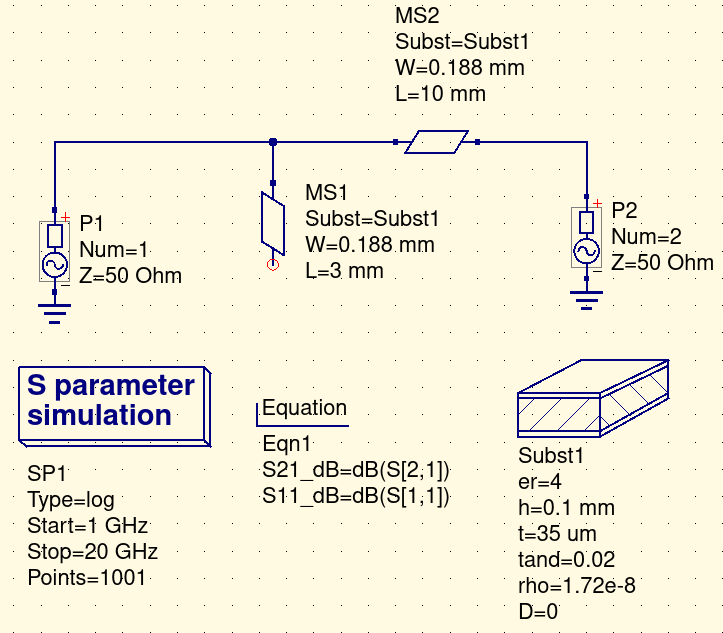
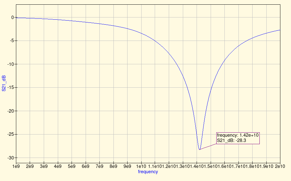
As advised by The Photon, I redid my calculation to compensate for the effect of an inhomogeneous microstrip surrounded by air. To do this, rather than using the \$ \epsilon_{r} \$ of the substrate, the effective relative permittivity \$ \epsilon_{r_{eff}} \$ should be used.

Rule-of-Thumb

First, I used a quick estimation I found online.

$$ \epsilon_{r_{eff}} = 0.64 \epsilon_{r} + 0.36 $$

It gives a resonant frequency of \$ f = \frac{c}{4l\sqrt{\epsilon_{reff}}} = 14.6 \text{GHz} \$, not too bad for a ballpark figure!

Hammerstad and Jensen

Next, I used the estimation by Hammerstad and Jensen, et al., found online from the textbook Microwave and RF design, a Systems Apporach, page 223 (Later I noticed Qucs also included this model, and actually the Schneider model is much easier to use than Hammerstad and Jensen, the formula is significantly shorter, but I already finished the original calculation at this point, sigh...)

Given \$ \epsilon_{r} \$, \$ w \$, and \$ h \$, Hammerstad and Jensen says the effective relative permittivity is:

$$ \epsilon_{r_{eff}} = \frac{\epsilon_r + 1}{2} + \frac{\epsilon_r - 1 }{2} (1 + \frac{10h}{w})^{-ab} $$

where

$$ u = \frac{w}{h} $$

$$ a(u) = 1 + \frac{1}{49} \ln[{\frac{u^4 + (u/52)^2}{u^4 + 0.432}}] + \frac{1}{18.7} \ln{[1+(\frac{u}{18.1})^3]} $$

$$ b(\epsilon_r) = 0.564 (\frac{\epsilon_r - 0.9}{\epsilon_r + 3})^{0.053} $$

Note that \$ u = \frac{w}{h} \$ is a dimensionless number, so absolute unit of measurement is irrelevant. The formula shows \$ \epsilon_{r_{eff}} = 3.05 \$ for my microstrip. Thus the resonant frequency \$ f = \frac{c}{4l\sqrt{\epsilon_{reff}}} = 14.3 \text{GHz} \$. It's exactly what the simulation shows.

Modeling for Fringing Effects

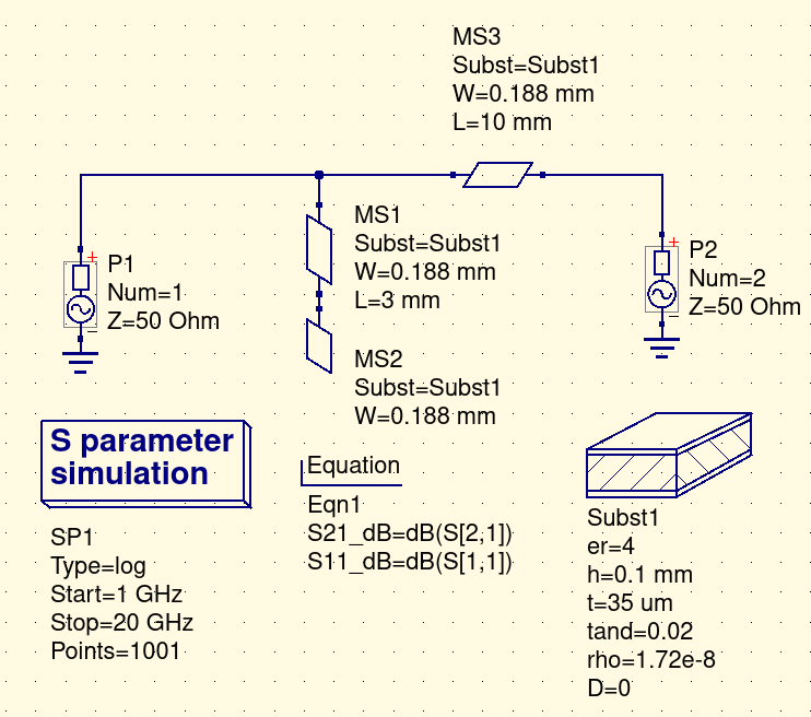
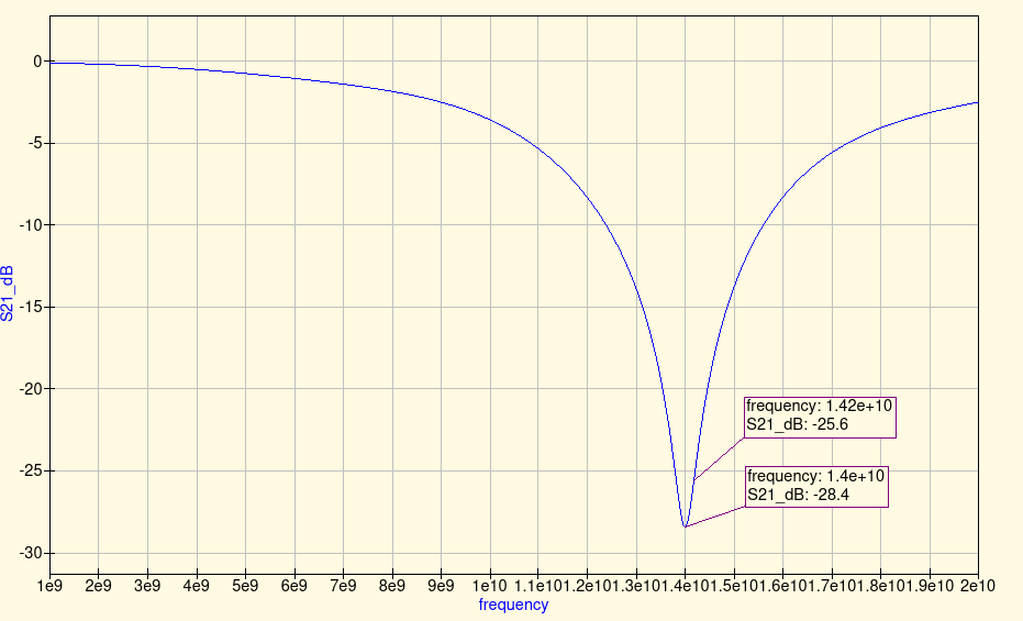
I also redid the simulation after connecting the open end of the "microstrip" to a "microstrip open" following The Photon's suggestions.

So after considering the fringing effects, a more realistic resonant frequency is 14.0 GHz.

Python code

For me to copy-paste in the future...

import math

def er_eff(er, w, h):
    u = w / h
    a = 1 + (1 / 49) * math.log((u ** 4 + (u / 52) ** 2) / (u ** 4 + 0.432)) + (1 / 18.7) * math.log(1 + (u / 18.1) ** 3)
    b = 0.564 * ((er - 0.9) / (er + 3)) ** 0.053
    return (er + 1) / 2 + ((er - 1) / 2) * (1 + (10 * h) / w) ** (-a * b)

>>> er_eff(4, 0.188, 0.1)
3.0544624555012434