2
\$\begingroup\$

For my power system, let us suppose it has the following dynamic model: \$\ x ' = f(x,u)\$.

This dynamic model consists of four first order differential equations (see below).

Then, I linearized my system using Newton-Raphson method. My new linear system will be:

\$\ \Delta x ' = A \Delta x + B u +\$ disturbance

Where:

  • \$\ x \$ is the state vector that that contains 4 first order differential equations: (the power angle δ , the angular speed of the rotor ω, the generated voltage in the quadrature axis of the generator eq', and the field voltage of the generator in the direct axis \$\ E_d\$ ). a.k.a.: \$\ \Delta x = [\Delta \delta, \Delta \omega. \Delta e_q' , \Delta E_d ] ^T \$

  • \$\ u \$ is the control part. Let us make it zero for now

  • Let us assume that the disturbance in the power input of the generator is just 30% (0.3 pu) for only 1 second.
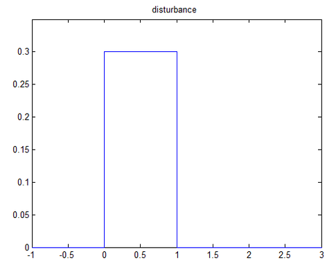
enter image description here

  • "A" is a 4 x 4 matrix. Let us say:

$$ A= \begin{bmatrix}1 & 2 & 3 &4\\5 & 6 &7 &8 \\9 & 1 & 2 & 3\\4 & 5 & 6 & 7 \end{bmatrix} $$

The question is:

How can I model the system shown above using MATLAB? I want to plot the four state variables, but I don't know where to begin

Is there any specific code that will help me to simulate this system.

\$\endgroup\$
1
  • \$\begingroup\$ Not sure what exactly you want to achieve, but usually the trick to modeling is staring with the errors (disturbance?) and then building it up backwards. \$\endgroup\$ Commented Feb 4, 2013 at 13:15

1 Answer 1

2
\$\begingroup\$

To solve this problem you should look at the ODE solvers in MATLAB.

Note that your function does not describe what the response of the system is to a variation in input power Pm.

Below I have written up an implementation, based on the example in http://www.its.caltech.edu/~ae121/ae121/ode45_Ref2.pdf . In my example I have added a term Pm to the differential equations, so you can see how a disturbance might affect the dynamics.

Unfortunately I don't have MATLAB installed so I can't check whether there are any errors in this, but the idea should be clear.

function main 
% a simple example to solve ODE's
% Uses ODE45 to solve 
%    dx_dt(1) = 1*x(1)+2*x(2)+3*x(3)+4*x(4)
%    dx_dt(2) = 5*x(1)+6*x(2)+7*x(3)+8*x(4)+Pm
%    dx_dt(3) = 9*x(1)+1*x(2)+2*x(3)+3*x(4)
%    dx_dt(4) = 4*x(1)+5*x(2)+6*x(3)+7*x(4)
%set an error
options=odeset('RelTol',1e-6);

%initial conditions
X0 = [0;0;0;0]; 
Pm0=1;

%before disturbance
tspan1 = [-1,0]; 
[t1,X1] = ode45('system',tspan1,X0,options,Pm0);

%during disturbance
tspan2 = [0,1];
[t2,X2] = ode45('system',tspan2,X1(end),options,1.3*Pm0);

%after disturbance
tspan3 = [1,3];
[t3,X3] = ode45('system',tspan3,X2(end),options,Pm0);

time=[t1,t2,t3];
X=[X1,X2,X3];

%plot the results
figure 
hold on
plot(time,X)
legend('x1','x2','x3','x4');ylabel('x');xlabel('t') 
return

%%%%%%%%%%%%%%%%%%%%%%%%%%%%%%%%%%%%%%%%%%%%%%%%%%%%%%%%%%
function [dx_dt]= system(t,x,Pm) 
%a function which returns a rate of change vector
A = [1,2,3,4;
     5,6,7,8;... 
     9,1,2,3;
     4,5,6,7]
P=[0;Pm;0;0]
dx_dt = A*x+P; 
return
\$\endgroup\$

Your Answer

By clicking “Post Your Answer”, you agree to our terms of service and acknowledge you have read our privacy policy.

Not the answer you're looking for? Browse other questions tagged or ask your own question.