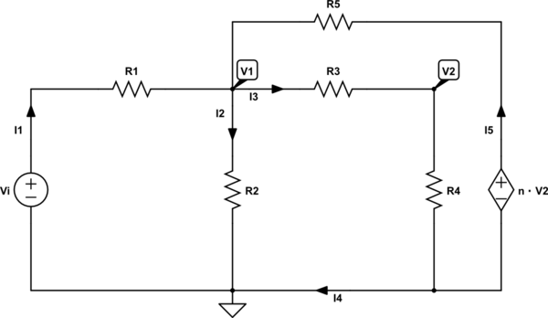
Well, we are trying the analyze the following circuit:
simulate this circuit – Schematic created using CircuitLab
When we use and apply KCL, we can write the following set of equations:
$$
\begin{cases}
\begin{alignat*}{1}
\text{I}_1+\text{I}_5&=\text{I}_2+\text{I}_3\\
\\
\text{I}_1&=\text{I}_2+\text{I}_4\\
\\
\text{I}_3&=\text{I}_4+\text{I}_5
\end{alignat*}
\end{cases}\tag1
$$
When we use and apply Ohm's law, we can write the following set of equations:
$$
\begin{cases}
\begin{alignat*}{1}
\text{I}_1&=\frac{\displaystyle\text{V}_\text{i}-\text{V}_1}{\displaystyle\text{R}_1}\\
\\
\text{I}_2&=\frac{\displaystyle\text{V}_1-0}{\displaystyle\text{R}_2}\\
\\
\text{I}_3&=\frac{\displaystyle\text{V}_1-\text{V}_2}{\displaystyle\text{R}_3}\\
\\
\text{I}_3&=\frac{\displaystyle\text{V}_2-0}{\displaystyle\text{R}_4}\\
\\
\text{I}_5&=\frac{\displaystyle\text{n}\cdot\text{V}_2-\text{V}_1}{\displaystyle\text{R}_5}
\end{alignat*}
\end{cases}\tag2
$$
Now, we can subsitute \$\displaystyle\left(2\right)\$ into \$\displaystyle\left(1\right)\$ in order to rewrite \$\displaystyle\left(1\right)\$:
$$
\begin{cases}
\begin{alignat*}{1}
\frac{\displaystyle\text{V}_\text{i}-\text{V}_1}{\displaystyle\text{R}_1}+\frac{\displaystyle\text{n}\cdot\text{V}_2-\text{V}_1}{\displaystyle\text{R}_5}&=\frac{\displaystyle\text{V}_1-0}{\displaystyle\text{R}_2}+\frac{\displaystyle\text{V}_1-\text{V}_2}{\displaystyle\text{R}_3}\\
\\
\frac{\displaystyle\text{V}_\text{i}-\text{V}_1}{\displaystyle\text{R}_1}+\frac{\displaystyle\text{n}\cdot\text{V}_2-\text{V}_1}{\displaystyle\text{R}_5}&=\frac{\displaystyle\text{V}_1-0}{\displaystyle\text{R}_2}+\frac{\displaystyle\text{V}_2-0}{\displaystyle\text{R}_4}\\
\\
\frac{\displaystyle\text{V}_\text{i}-\text{V}_1}{\displaystyle\text{R}_1}&=\frac{\displaystyle\text{V}_1-0}{\displaystyle\text{R}_2}+\text{I}_4\\
\\
\frac{\displaystyle\text{V}_1-\text{V}_2}{\displaystyle\text{R}_3}&=\text{I}_4+\frac{\displaystyle\text{n}\cdot\text{V}_2-\text{V}_1}{\displaystyle\text{R}_5}\\
\\
\frac{\displaystyle\text{V}_2-0}{\displaystyle\text{R}_4}&=\text{I}_4+\frac{\displaystyle\text{n}\cdot\text{V}_2-\text{V}_1}{\displaystyle\text{R}_5}
\end{alignat*}
\end{cases}\tag3
$$
Now, you can use Laplace transform to write:
$$\text{R}_2=\frac{\displaystyle1}{\displaystyle\text{sC}},\space\text{R}_3=\text{sL}\tag4$$
And:
$$\text{v}_\text{i}\left(\text{s}\right)=\mathscr{L}_t\left[\hat{\text{u}}_\text{i}\cos\left(\omega t\right)\right]_{\left(\text{s}\right)}=\frac{\displaystyle\hat{\text{u}}_\text{i}\text{s}}{\displaystyle\text{s}^2+\omega^2}\tag5$$
Now, for your case you need to solve for \$\displaystyle-\text{I}_5\$ in order to find your \$\displaystyle i_o\$.
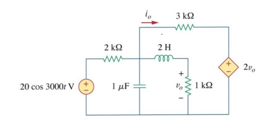 For the above question, after solving the circuit in frequency domain, I got the value of $$i_0(t) = 1.14\cos(3000t-55.3) mA $$ approximately (The calculations in the middle of steps was not approximated.)
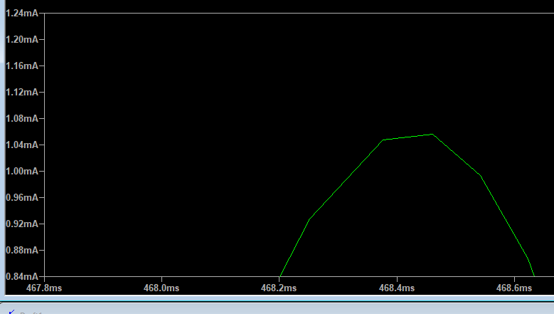 The peak is approximately 1.056 mA of the current. There is a slight difference between the theoretical value and the value LTspice displays.
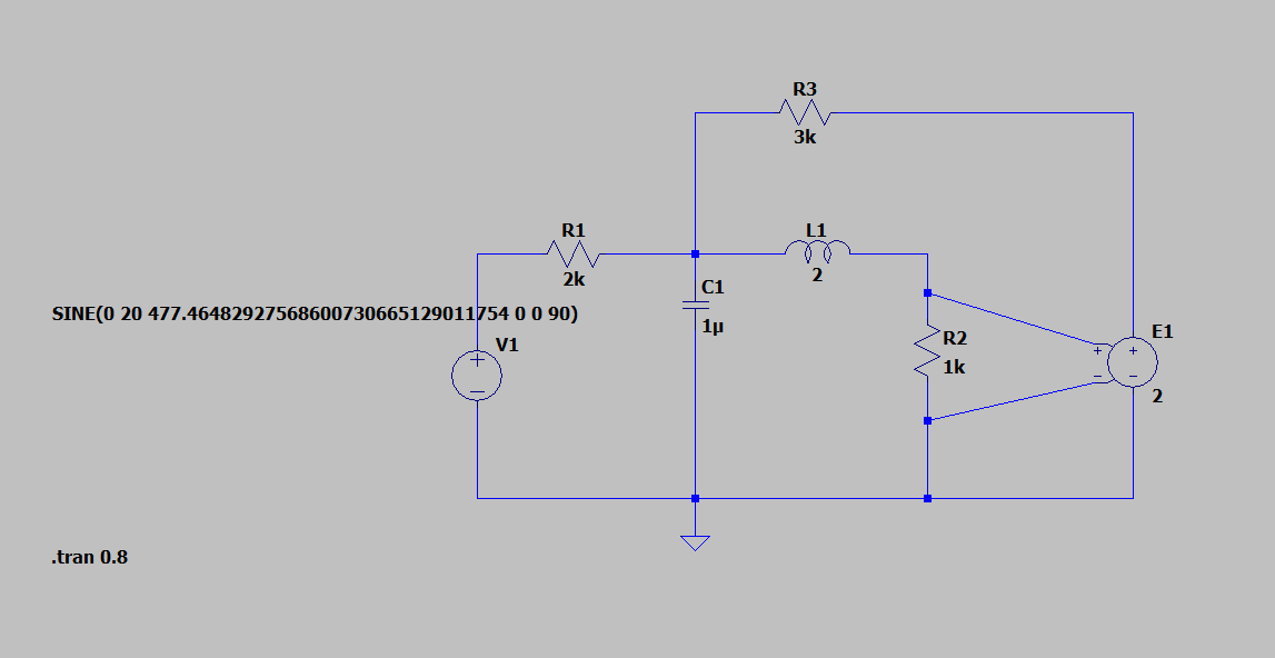


.tran 0 0.8 0 1u\$\endgroup\$.OPTION PLOTWINSIZE=0card. And Spice programs take many shortcuts. In short, don't expect perfection when running simulators. That is expecting too much from them. \$\endgroup\$