LTspice issues with op-amp filter

Question

I need to simulate in LTspice a wattmeter connected to a 800 V DC/DC converter (step-down) with silicon carbide (SiC) transistors. The wattmeter measures the voltage across the lower transistor (V_out) and the inductor current, but we'll focus on V_out for my question. The goal is to study the differences before and after the filter, to calculate losses in the semiconductors in a real experiment.

The wattmeter is simply modeled as a Bessel low-pass filter (cut-off frequency of 150 kHz approx.). I know the transfer function of the filter.

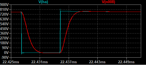
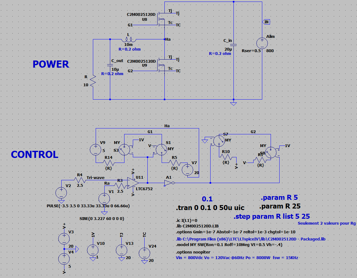
The DC/DC converter has yet been modelized and the simulation works well. This simulation comes from the SiC transistors manufacturer's website. The simulation parameters have been optimized. V_out (Ha potential) looks like a square wave, with oscillations and overshoots caused by commutations.

First, I've tried to create the filter using a "voltage controlled voltage source", where I put the Laplace function:

I integrated this filter in the DC/DC converter simulation and it seemed to work nicely:

But if we look closely to the 2 signals after a time long enough after a commutation, there is a static error of 400 mV between them. Which is weird because the gain of the transfer function is equal to 1.

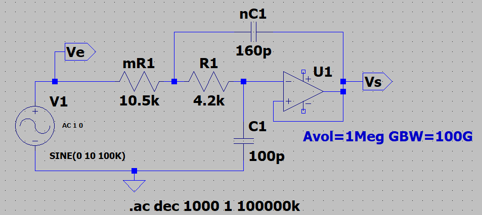
So, I tried to model the filter using an amp-op (Sallen-Key topology):

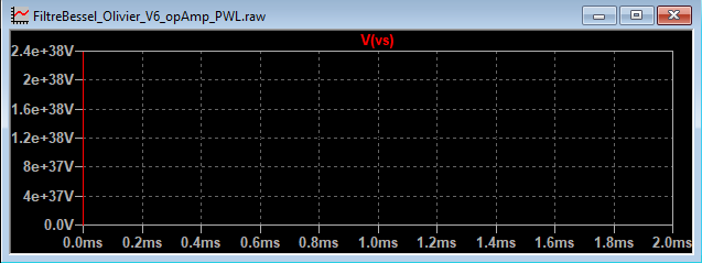
In the simulation, I choose an ideal Op-Amp level 1 (parameters: Avol=1Meg; GBW=100G; Vos=0; En=0; Enk=0; Ink=0; Rin=500Meg). This filter works well with an ideal square voltage source, but it doesn’t work at all when I connect the filter to the DC/DC converter. The simulation has become infinitely slow (simulation speed around 1 femtos/s). Then, I simulate the converter alone, without the filter, and I saved V_out in a file, using “export data as text”. I opened a new simulation, with the filter connected to a PWL voltage source which received the text file. The simulation runs but the output voltage of the filter is wrong - infinite :

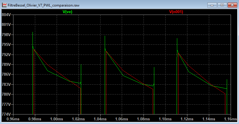
And there is another issue: the PWL signal is not exactly the same that the signal which was used to create the text file:

I would really appreciate your help and I thank you in advance. If my problem is unclear, I can reformulate. Sorry for my English...

PS: I sometimes get errors like "Singular matric: check nodes xxx and yyy iteration no.2"

Answer 1

You have two separate problems going on here. First, there is an issue with your Sallen-Key circuit that Carl Rutschow already pointed out in your question's comments. Restating, the inputs of your opamp are flipped. You want the direct feedback from output to (-) instead of output to (+), as shown on Wikipedia.

Your main problem, which got you down the path of making the Sallen-Key circuit in the first place, has to do with the Laplace feature of LTspice. Laplace is meant to mainly be used in the frequency domain (i.e. an .ac analysis). This makes sense, since the s-domain is a frequency domain and it's evaluated directly in terms of frequency by the SPICE engine. Your results agree with this. However, when you moved to the time domain, you started to have problems. So what does LTspice do when it has to evaluate your Laplace expression in the time domain? Similar to what you do/did in school, it needs to calculate the inverse Laplace transform to find the impulse response so it can perform a convolution with your input to get the output. It approximates this inverse transform using an FFT, and it auto-calculates the window length (Window keyword) and FFT size (Nfft keyword) required to get a good fit. The LTspice built-in help for B. Arbitrary Behavioral Voltage or Current Sources explains this much better:

If an optional Laplace transform is defined, that transform is applied to the result of the behavioral current or voltage. The Laplace transform must be a function solely of s. The Boolean XOR operator, ^, is understood to mean exponentiation, **, when used in a Laplace expression. The frequency response at frequency f is found by substituting s with sqrt(-1)2pi*f. The time domain behavior is found from the sum of the instantaneous current(or voltage) with the convolution of the history of this current(or voltage) with the impulse response. Numerical inversion of a Laplace transfer function to the time domain impulse response is a potentially compute-bound process and a topic of current numerical research. In LTspice, the impulse response is found from the FFT of a discrete set points in frequency domain response. This process is prone to the usual artifacts of FFT's such as spectral leakage and picket fencing that is common to discrete FFT's. LTspice uses a proprietary algorithm that exploits that it has an exact analytical expression for the frequency domain response and chooses points and windows to cause such artifacts to diffract precisely to zero. However, LTspice must guess an appropriate frequency range and resolution. It is recommended that the LTspice first be allowed to make a guess at this. The length of the window and number of FFT data points used will be reported in the .log file. You can then adjust the algorithm's choices by explicitly setting nfft and window length. The reciprocal of the value of the window is the frequency resolution. The value of nfft times this resolution is the highest frequency considered. Note that the convolution of the impulse response with the behavioral source is also potentially a compute bound process.

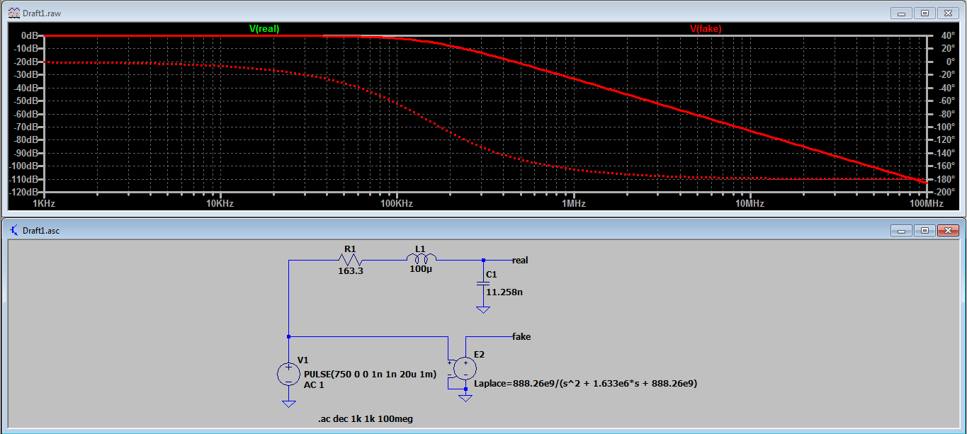
I don't know how you calculated your transfer function, so I made my own and compared it to an equivalent 2nd order RLC lowpass filter circuit. When you run an .ac analysis the plots line up exactly (red trace completely covers green trace).

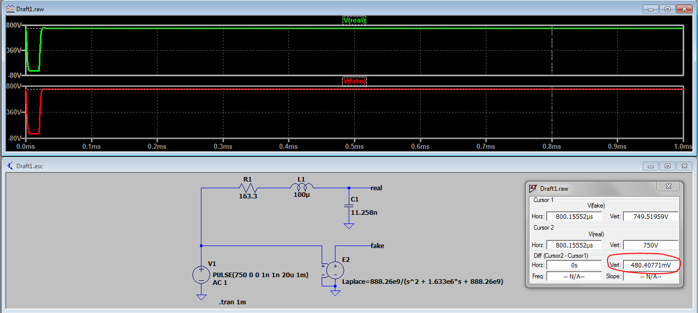
Now, comparing these in the time domain using .tran there shows a discrepancy after the pulse settles. The screenshot below shows a 480.41mV discrepancy.

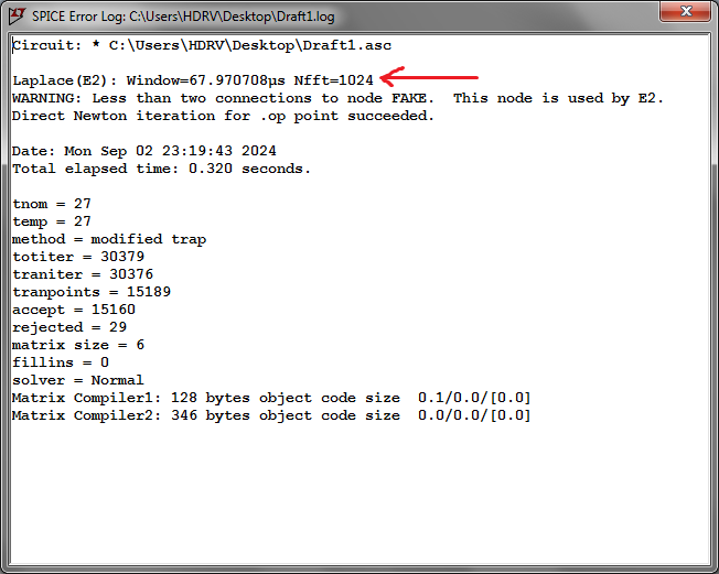
If you pull up the SPICE Error Log CTRL+L, it shows you the values LTspice used for Window and Nfft.

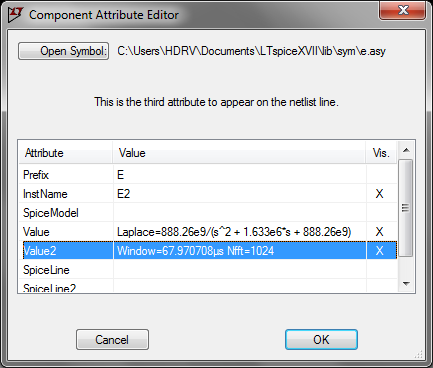
You can use these as a starting point by copy/pasting them into your E-source definition, as shown.

However, I never really ever had success in adjusting LTspice's auto-calculated values for a Laplace FFT. You can try it regardless, and see what happens. The moral of the story is to know that Laplace has limitations when used for the time domain. It's good to be aware of this since Laplace can be useful, but avoid using it in the time domain whenever you can.