added 16 characters in body
Source Link
CroCo
  • 328
  • 2
  • 14

In order to draw the root locus, you need to convert the open-loop system into the closed-loop system. You can do this

$$ \begin{align} T(s) &= \frac{ \frac{1}{(s+3)(s+4)} }{ 1+ \frac{1}{(s+3)(s+4)} \frac{K}{s(s+1)} } \\ &= \frac{s^2+s}{s^4+8s^3+19s^2+12s+K} \end{align} $$ Now the gain K appears in the characteristic equation of the closed-loop \$T(s)\$ (i.e the denominator). You can easily vary K from 0 to infinity to compute the poles of the characteristic equation of the closed-loop \$T(s)\$ using any software (e.g. Matlab). If the gain K is zero, we have these poles 0,-1,-3,-4. Use this Matlab script to compute the poles at different gains

K=0; % vary it from 0 to big number
poles = roots([1 8 19 12 K])

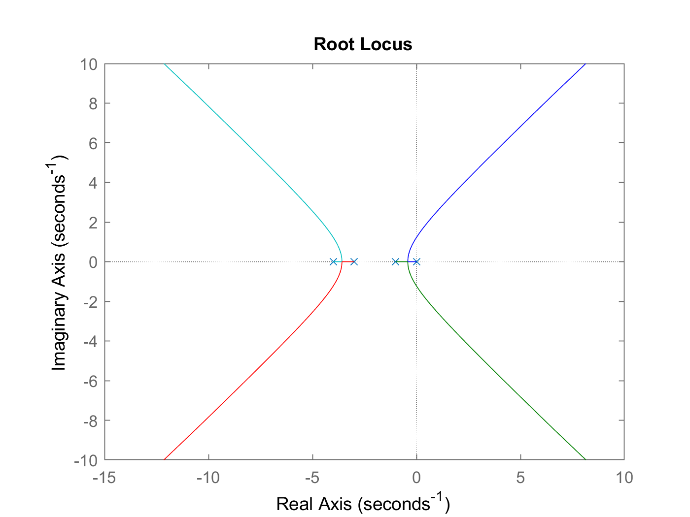
You just need tabular data to plot the root locus. You may use Matlab as well.

GH=zpk([],[0 -1 -3 -4],1);
sys=tf(GH);
rlocus(GH)

Or this elegant code

s=tf('s');
G = 1/((s+3)*(s+4));
H = 1/(s*(s+1));
sys = G*H;
rlocus(G*Hsys)

enter image description here

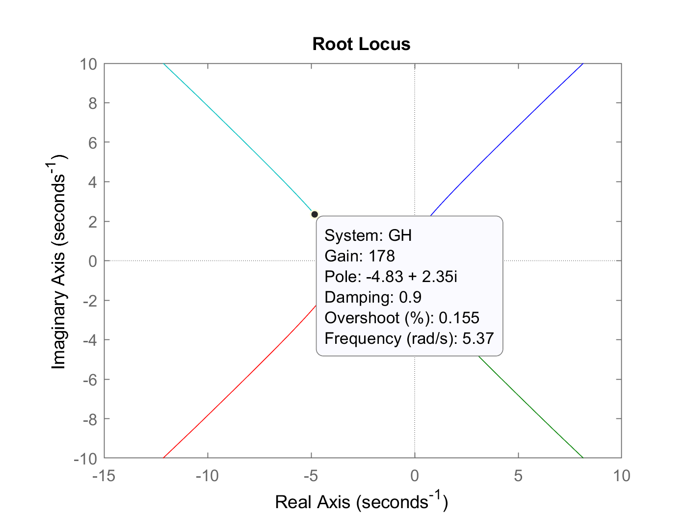
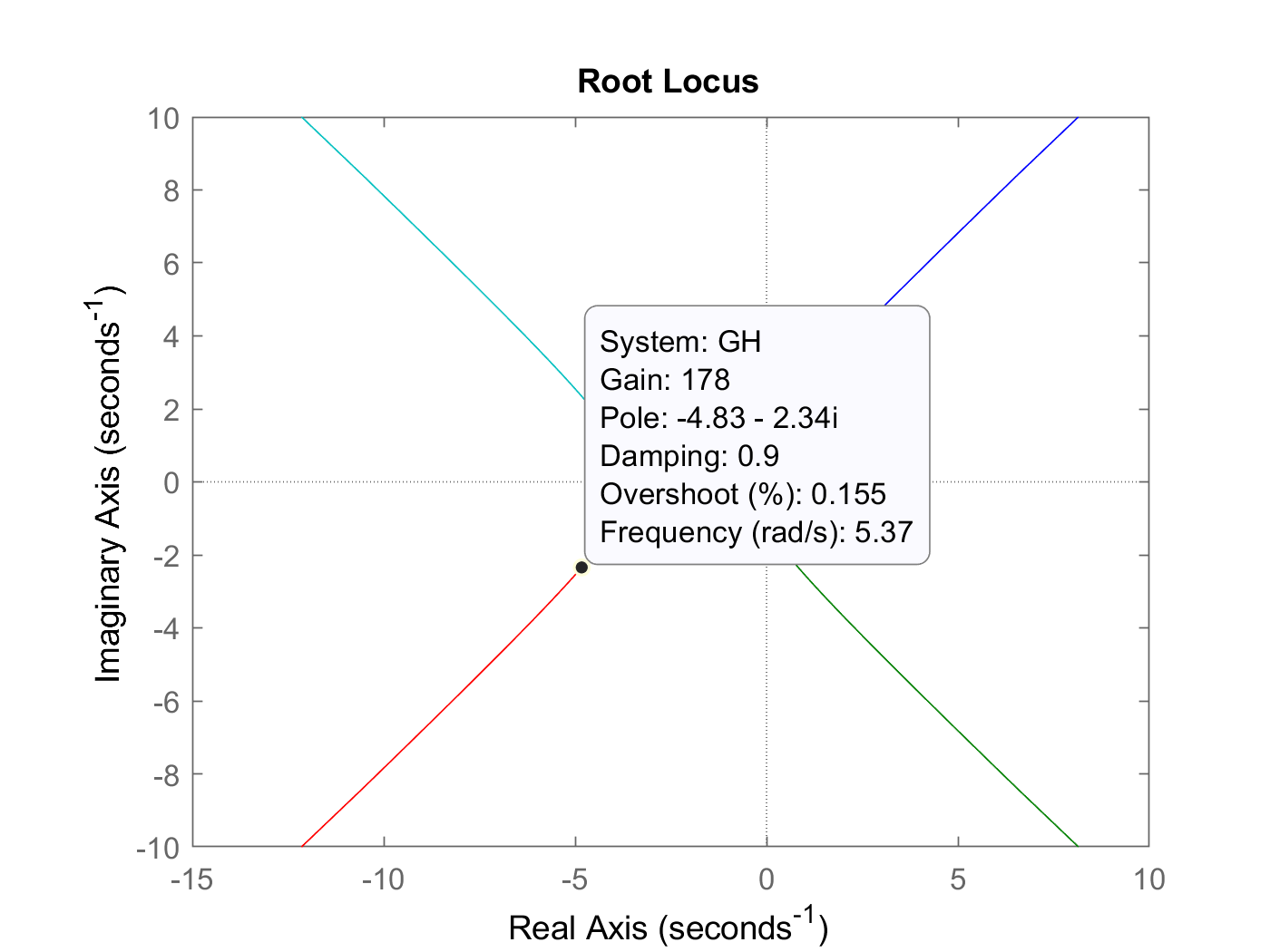
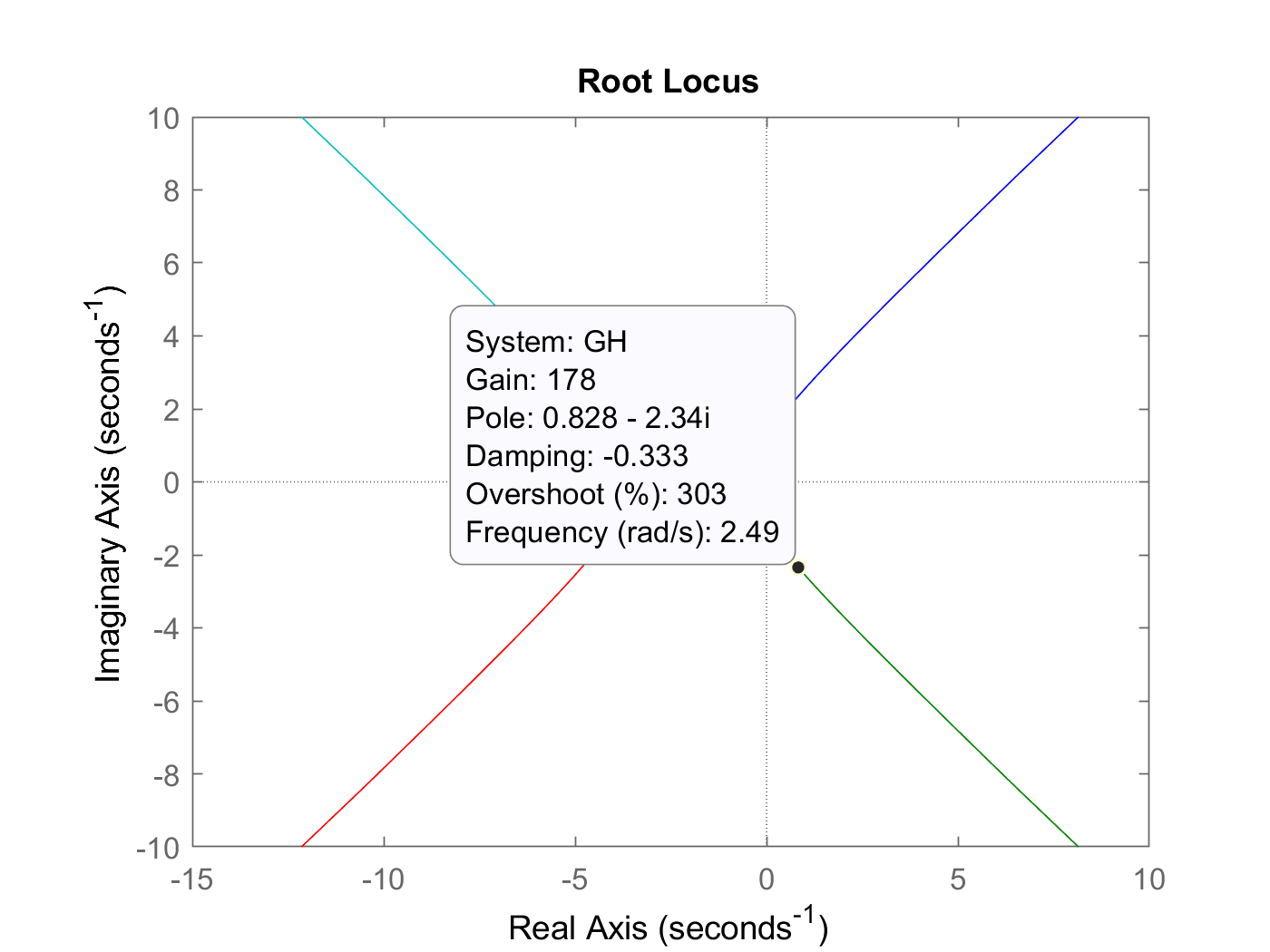
Let's go back to roots([1 8 19 12 K]) if K is 178, we have these poles

  -4.8276 + 2.3442i
  -4.8276 - 2.3442i
   0.8276 + 2.3442i
   0.8276 - 2.3442i

We can see same result in the root locus obtained by Matlab at this gain,

enter image description here enter image description here enter image description here

In order to draw the root locus, you need to convert the open-loop system into the closed-loop system. You can do this

$$ \begin{align} T(s) &= \frac{ \frac{1}{(s+3)(s+4)} }{ 1+ \frac{1}{(s+3)(s+4)} \frac{K}{s(s+1)} } \\ &= \frac{s^2+s}{s^4+8s^3+19s^2+12s+K} \end{align} $$ Now the gain K appears in the characteristic equation of the closed-loop \$T(s)\$ (i.e the denominator). You can easily vary K from 0 to infinity to compute the poles of the characteristic equation of the closed-loop \$T(s)\$ using any software (e.g. Matlab). If the gain K is zero, we have these poles 0,-1,-3,-4. Use this Matlab script to compute the poles at different gains

K=0; % vary it from 0 to big number
poles = roots([1 8 19 12 K])

You just need tabular data to plot the root locus. You may use Matlab as well.

GH=zpk([],[0 -1 -3 -4],1);
sys=tf(GH);
rlocus(GH)

Or this elegant code

s=tf('s');
G = 1/((s+3)*(s+4));
H = 1/(s*(s+1));
rlocus(G*H)

enter image description here

Let's go back to roots([1 8 19 12 K]) if K is 178, we have these poles

  -4.8276 + 2.3442i
  -4.8276 - 2.3442i
   0.8276 + 2.3442i
   0.8276 - 2.3442i

We can see same result in the root locus obtained by Matlab at this gain,
enter image description here enter image description here enter image description here

In order to draw the root locus, you need to convert the open-loop system into the closed-loop system. You can do this

$$ \begin{align} T(s) &= \frac{ \frac{1}{(s+3)(s+4)} }{ 1+ \frac{1}{(s+3)(s+4)} \frac{K}{s(s+1)} } \\ &= \frac{s^2+s}{s^4+8s^3+19s^2+12s+K} \end{align} $$ Now the gain K appears in the characteristic equation of the closed-loop \$T(s)\$ (i.e the denominator). You can easily vary K from 0 to infinity to compute the poles of the characteristic equation of the closed-loop \$T(s)\$ using any software (e.g. Matlab). If the gain K is zero, we have these poles 0,-1,-3,-4. Use this Matlab script to compute the poles at different gains

K=0; % vary it from 0 to big number
poles = roots([1 8 19 12 K])

You just need tabular data to plot the root locus. You may use Matlab as well.

GH=zpk([],[0 -1 -3 -4],1);
sys=tf(GH);
rlocus(GH)

Or this elegant code

s=tf('s');
G = 1/((s+3)*(s+4));
H = 1/(s*(s+1));
sys = G*H;
rlocus(sys)

enter image description here

Let's go back to roots([1 8 19 12 K]) if K is 178, we have these poles

  -4.8276 + 2.3442i
  -4.8276 - 2.3442i
   0.8276 + 2.3442i
   0.8276 - 2.3442i

We can see same result in the root locus obtained by Matlab at this gain,
enter image description here enter image description here enter image description here

added 170 characters in body
Source Link
CroCo
  • 328
  • 2
  • 14

In order to draw the root locus, you need to convert the open-loop system into the closed-loop system. You can do this

$$ \begin{align} T(s) &= \frac{ \frac{1}{(s+3)(s+4)} }{ 1+ \frac{1}{(s+3)(s+4)} \frac{K}{s(s+1)} } \\ &= \frac{s^2+s}{s^4+8s^3+19s^2+12s+K} \end{align} $$ Now the gain K appears in the characteristic equation of the closed-loop \$T(s)\$ (i.e the denominator). You can easily vary K from 0 to infinity to compute the poles of the characteristic equation of the closed-loop \$T(s)\$ using any software (e.g. Matlab). If the gain K is zero, we have these poles 0,-1,-3,-4. Use this Matlab script to compute the poles at different gains

K=0; % vary it from 0 to big number
poles = roots([1 8 19 12 K])

You just need tabular data to plot the root locus. You may use Matlab as well.

GH=zpk([],[0 -1 -3 -4],1);
sys=tf(GH);
rlocus(GH)

Or this elegant code

s=tf('s');
G = 1/((s+3)*(s+4));
H = 1/(s*(s+1));
rlocus(G*H)

enter image description here

Let's go back to roots([1 8 19 12 K]) if K is 178, we have these poles

  -4.8276 + 2.3442i
  -4.8276 - 2.3442i
   0.8276 + 2.3442i
   0.8276 - 2.3442i

We can see same result in the root locus obtained by Matlab at this gain,
enter image description here enter image description here enter image description here

In order to draw the root locus, you need to convert the open-loop system into the closed-loop system. You can do this

$$ \begin{align} T(s) &= \frac{ \frac{1}{(s+3)(s+4)} }{ 1+ \frac{1}{(s+3)(s+4)} \frac{K}{s(s+1)} } \\ &= \frac{s^2+s}{s^4+8s^3+19s^2+12s+K} \end{align} $$ Now the gain K appears in the characteristic equation of the closed-loop \$T(s)\$ (i.e the denominator). You can easily vary K from 0 to infinity to compute the poles of the characteristic equation of the closed-loop \$T(s)\$ using any software (e.g. Matlab). If the gain K is zero, we have these poles 0,-1,-3,-4. Use this Matlab script to compute the poles at different gains

K=0; % vary it from 0 to big number
poles = roots([1 8 19 12 K])

You just need tabular data to plot the root locus. You may use Matlab as well.

GH=zpk([],[0 -1 -3 -4],1);
sys=tf(GH);
rlocus(GH)

enter image description here

Let's go back to roots([1 8 19 12 K]) if K is 178, we have these poles

  -4.8276 + 2.3442i
  -4.8276 - 2.3442i
   0.8276 + 2.3442i
   0.8276 - 2.3442i

We can see same result in the root locus obtained by Matlab at this gain,
enter image description here

In order to draw the root locus, you need to convert the open-loop system into the closed-loop system. You can do this

$$ \begin{align} T(s) &= \frac{ \frac{1}{(s+3)(s+4)} }{ 1+ \frac{1}{(s+3)(s+4)} \frac{K}{s(s+1)} } \\ &= \frac{s^2+s}{s^4+8s^3+19s^2+12s+K} \end{align} $$ Now the gain K appears in the characteristic equation of the closed-loop \$T(s)\$ (i.e the denominator). You can easily vary K from 0 to infinity to compute the poles of the characteristic equation of the closed-loop \$T(s)\$ using any software (e.g. Matlab). If the gain K is zero, we have these poles 0,-1,-3,-4. Use this Matlab script to compute the poles at different gains

K=0; % vary it from 0 to big number
poles = roots([1 8 19 12 K])

You just need tabular data to plot the root locus. You may use Matlab as well.

GH=zpk([],[0 -1 -3 -4],1);
sys=tf(GH);
rlocus(GH)

Or this elegant code

s=tf('s');
G = 1/((s+3)*(s+4));
H = 1/(s*(s+1));
rlocus(G*H)

enter image description here

Let's go back to roots([1 8 19 12 K]) if K is 178, we have these poles

  -4.8276 + 2.3442i
  -4.8276 - 2.3442i
   0.8276 + 2.3442i
   0.8276 - 2.3442i

We can see same result in the root locus obtained by Matlab at this gain,

enter image description here enter image description here enter image description here

Source Link
CroCo
  • 328
  • 2
  • 14

In order to draw the root locus, you need to convert the open-loop system into the closed-loop system. You can do this

$$ \begin{align} T(s) &= \frac{ \frac{1}{(s+3)(s+4)} }{ 1+ \frac{1}{(s+3)(s+4)} \frac{K}{s(s+1)} } \\ &= \frac{s^2+s}{s^4+8s^3+19s^2+12s+K} \end{align} $$ Now the gain K appears in the characteristic equation of the closed-loop \$T(s)\$ (i.e the denominator). You can easily vary K from 0 to infinity to compute the poles of the characteristic equation of the closed-loop \$T(s)\$ using any software (e.g. Matlab). If the gain K is zero, we have these poles 0,-1,-3,-4. Use this Matlab script to compute the poles at different gains

K=0; % vary it from 0 to big number
poles = roots([1 8 19 12 K])

You just need tabular data to plot the root locus. You may use Matlab as well.

GH=zpk([],[0 -1 -3 -4],1);
sys=tf(GH);
rlocus(GH)

enter image description here

Let's go back to roots([1 8 19 12 K]) if K is 178, we have these poles

  -4.8276 + 2.3442i
  -4.8276 - 2.3442i
   0.8276 + 2.3442i
   0.8276 - 2.3442i

We can see same result in the root locus obtained by Matlab at this gain,

enter image description here