I need someone to check my understanding of Nyquist frequency. I understand it in the following manner.
$$F_{nyquist} = ( F_{sampling}/2 ) * n$$ where n is an integer (negative and positive). For instance:
$$ F_{sampling} = 10 kHz $$ then $$F_{nyquist} = [-10, -5, 0_{(?)}, 5, 10] kHz$$ I am not sure, whether 0 is a nyquist frequency (Question 1). Then the mirroring a.k.a detected alias frequencies can be found at the following locations:
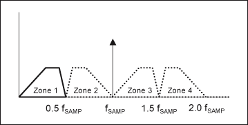
(\$F_s\$ in the picture is \$F_{sampling}\$)
- green - signal being sampled (original signal)
- red - alias frequencies
- yellow - is it alias frequency ? (Question 2)
Questions:
1) is F = 0 Nyquist frequency ?
2) does the mirroring happens around F = 0 ?
3) is my understanding correct ? Are the red circles alias frequencies ?
The problem is, that I cant replicate all of the alias frequencies in matlab. I can see alias at $$ F_{alias} = F_{sampling}*n + F_{signal}$$. For signal at $$F_{signal} = 3 kHz$$ I can see aliases at $$F_{alias} = [13, 23, 33]$$
 , but I DONT see it at $$F_{alias} = [7, 17, 27]$$ as expected due to the mirroring.
The following MATLAb code should illustrate the process I understand as "looking" for aliases.
clear all;
clc;

% sampling rate
F_sample = 10000;
T = 1 / F_sample;
% time range
t = [0:T:T*10];         % asmpling time - 10 samples
t_x = [0:T/100:T*10];   % smooth "time" to see the sinusoids of F_aliases signlas

% nyquist frequency
F_nyquist = F_sample / 2;

% arbitrary signal within sampling range (F_signal is less than F_sample / 2)
F_signal = 3000;

% when the following frequencies are sampled, they should appear as the
% F_signal
F_alias_1 = F_nyquist*2 - F_signal; % 1st mirroring - Zone 2
F_alias_2 = F_nyquist*2 + F_signal; % 2nd mirroring - Zone 3

% from F to w
w_signal = 2*pi*F_signal;
w_alias_1 = 2*pi*F_alias_1;
w_alias_2 = 2*pi*F_alias_2;

% calculate signals
x1 = sin(w_signal*t);       % samples (red circles)
x2 = sin(w_alias_1*t_x);    % blue signal
x3 = sin(w_alias_2*t_x);    % green signal

plot(t,x1,'ro');      % Sampling (red circles)
hold on;
plot(t_x,x2,'b');     % 1st frequency that SHOULD be sampled the same as original signal
hold on;
plot(t_x,x3,'g');     % 2nd frequency that SHOULD be sampled the same as original signal

xlabel('time');
ylabel('amplitude');
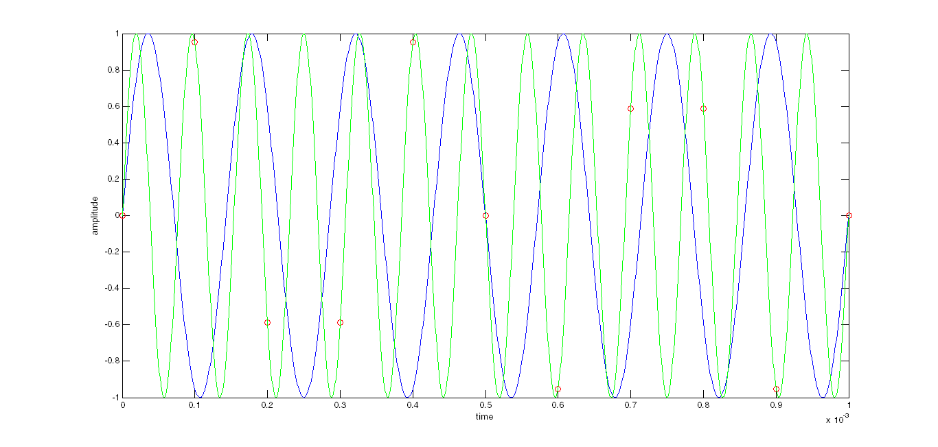
- red circles - samples of 3 kHz signal at 10 kHz sampling rate (original signal at 3kHz is not depicted, just its samples)
- blue - alias at 7 kHz (1st above 5 kHz (Zone 2), half of sampling frequency)
- green - alias at 13 kHz (2nd above 5 kHz (Zone 3), half of sampling frequency)
Obviously, the blue doesnt "fit" the samples, while the green fit them perfectly


