4
\$\begingroup\$

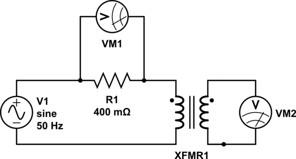
I am trying to measure the magnetic hysteresis curve of a toroidal nanocrystalline ferromagnetic transformer core made of Nanoperm (datasheet linked) using the following circuit. Each of the windings (primary on input side and secondary on measurement side) has 6 turns of 16 AWG magnet wire. The 1 micro-F capacitor on the output side is used because when the magnetic field saturates, the output current goes to zero. Thus, with just an RL circuit on the measurement side, the voltage drop across both the coil and the 5 kOhm resistor are zero during saturation. The capacitor essentially holds the saturation voltage until the polarity of the input is reversed.

I justified my method first intuitively and later confirmed that it more or less matched with the method shown here (section title: "Measuring arrangement with an analog oscilloscope"). The only difference is that rather than directly connecting the function generator to the primary coil and using an op-amp integrator circuit on the measurement side, I use an audio amplifier (not shown) to amplify the current of the function generator to approximately 5.3 A (= 2.1 V / 0.4 ohms) and use a passive integrator on the measurement side.
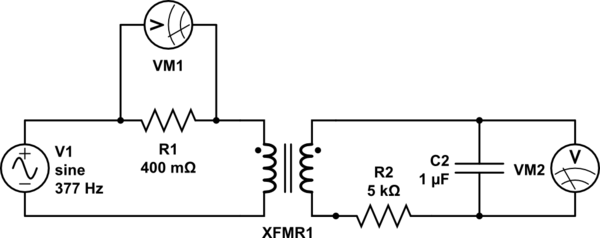
schematic

simulate this circuit – Schematic created using CircuitLab

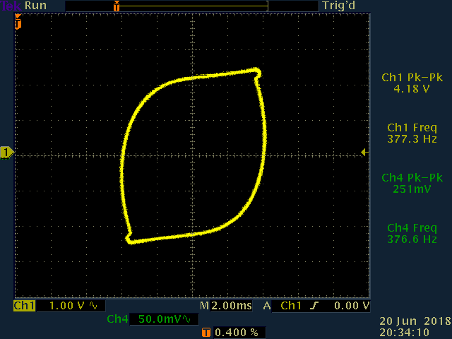
An image of the hysteresis curved as measured on my oscilloscope is shown below. VM1 is plotted on the horizontal axis, and VM2 is plotted on the vertical axis.

enter image description here

Based on this information, how can I calculate (Q1-1) the magnetic field strength (in A/m) applied to and (Q1-2) the magnetic flux density (in T) induced in the core up to and during saturation?


UPDATE (8/6/18, 4:00 a.m.): In response to comments by @glen_geek, I re-did my experiment and made two changes. My questions are in bold and are marked as (Q2-X).

First, I realized that it was a mistake to use a single-ended probe for VM1 (with the ground side placed at the node between the resistor and the coil on the transformer). The resistor has a resistance of 400 mOhms, and the coil has a resistance of 200 mOhms. When signal is passing through the coils, the impedance will increase further since \$Z = \sqrt{R^2 + (\omega L)^2}\$. By placing the ground side of the probe there, I was incorrectly grounding my signal where it should not have been. I was using a differential probe for VM2, but I only have one differential probe that plugs into my oscilloscope. However, I have a NIDAQ which can record up to 40 differential inputs, so I decided to use it to probe the voltages across R1 and C2 and stopped using the standalone oscilloscope.

Next, as suggested by @glen_geek, I increased the resistance of R2, first up to 10 kOhms and then up to 27 kOhms and 37 kOhms. (Q2-1) It is still unclear to me why we increase rather than decrease R2 because the cutoff frequency of the filter only gets smaller as we increase the resistance. If someone could clarify for me why this is helpful, I would appreciate it. (I understand that the higher the resistance, the lower the cutoff frequency; and the lower the cutoff frequency, the greater the window of integration since (1) the time constant gets larger and (2) a larger time constant implies a larger window over which the signal is smoothed, which is what is required for only lower frequencies to be passed. I'm just not sure why reducing the gain of the frequency of interest, which is much higher than the cutoffs tabulated below, is a good thing in this case.) (Q2-2) Furthermore, is it even reasonable to use any gain other than 1 unless we compensate for it when we calculate the field strength and/or flux density?

Based on the datasheets shown here (page 3) and here, I found that the manufacturers quantified the hysteresis at 50 Hz. To try and replicate their results, I decided to run my experiment at 50 Hz as well. I also decided to run it at 350 Hz and at 380 Hz, which is close to the 377 Hz I was using before. (@glen_geek, you mentioned in your comment that it was suspicious that \$\omega = 377\$. In fact, \$f\$ was \$377\$ Hz, not \$\omega\$, which is \$2\pi f = 2\pi(377) = 2368\$ rad/s.)

The table below summarizes the cutoff frequencies and gains for input frequencies of 350 and 50 Hz, which were used in these experiments: enter image description here

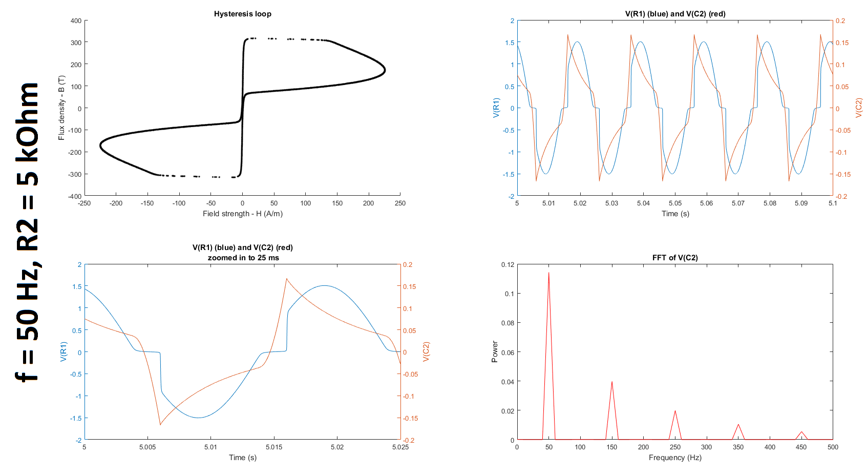
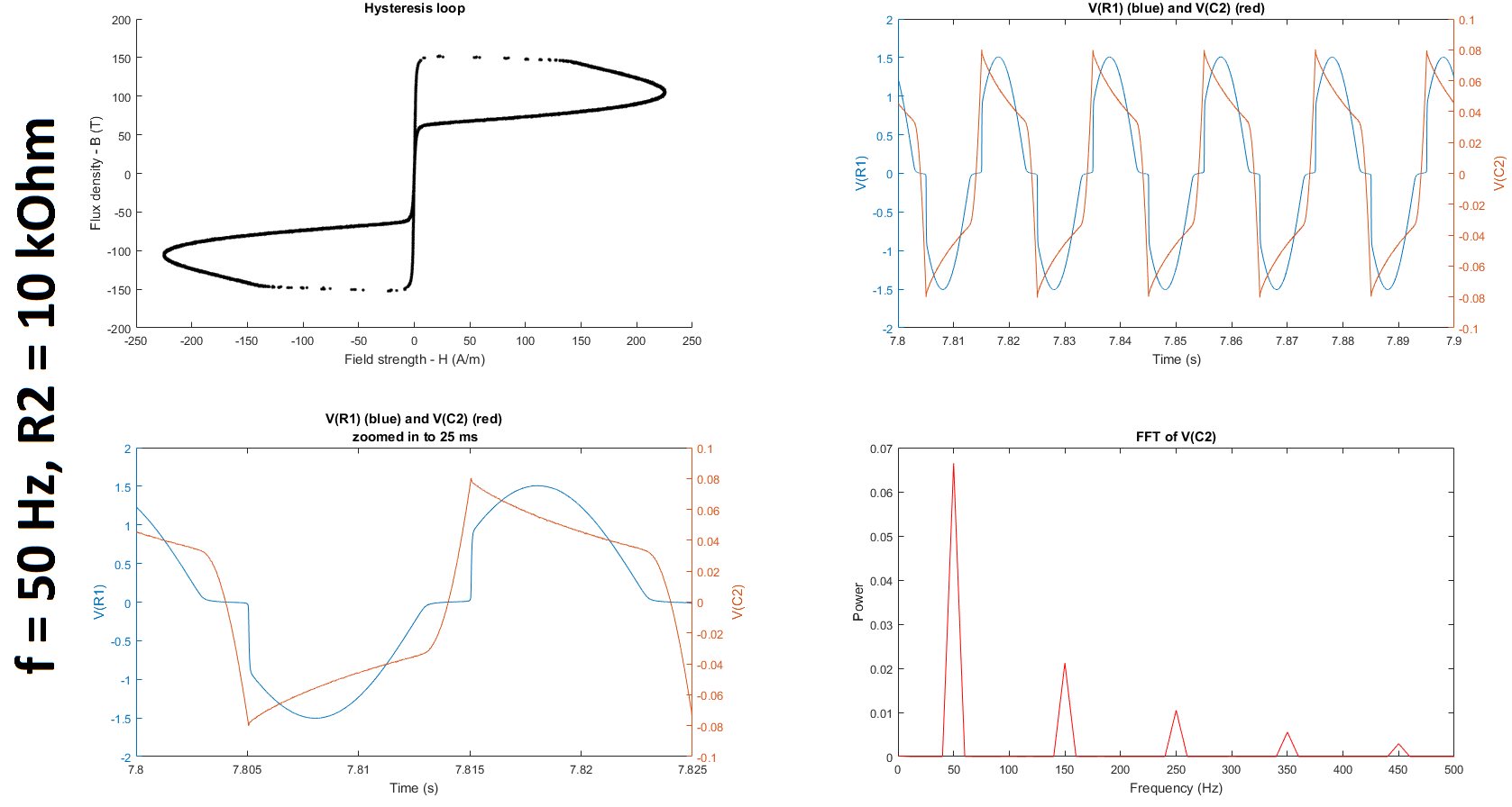
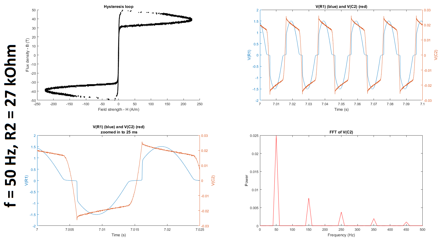
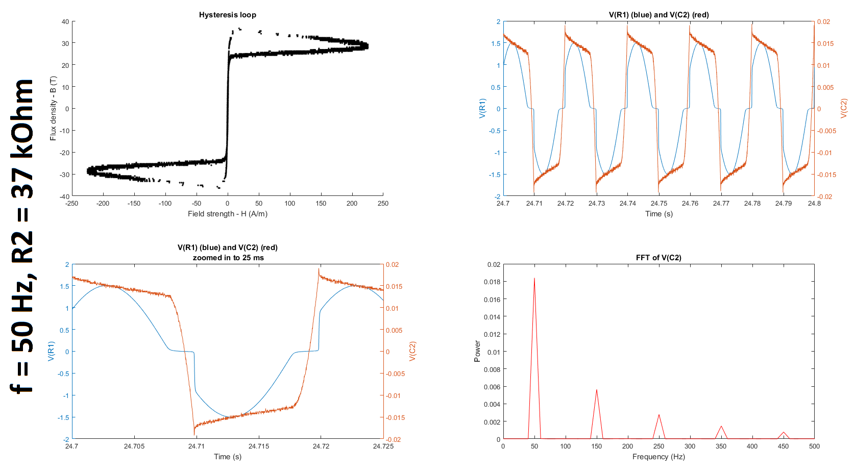
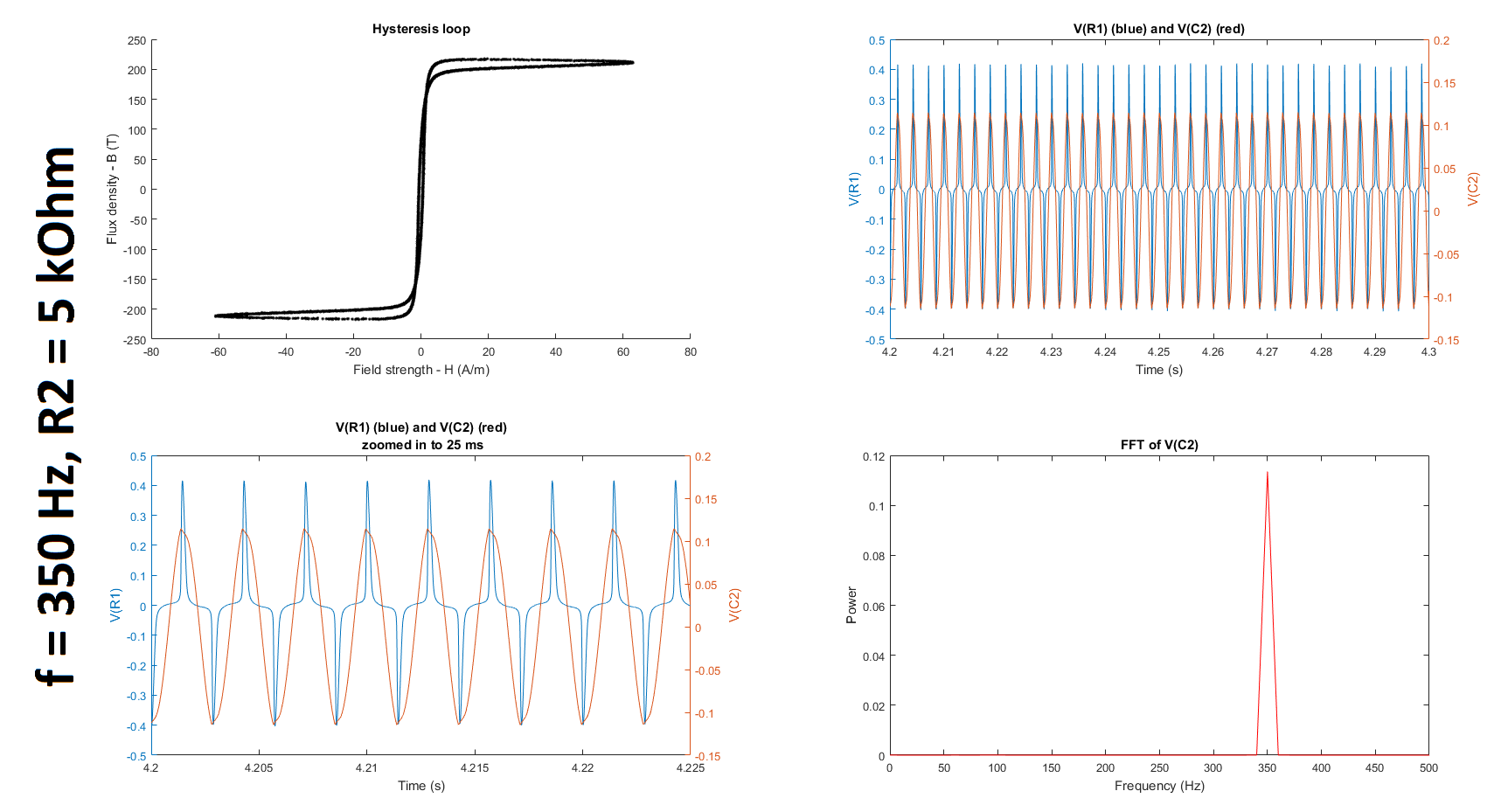
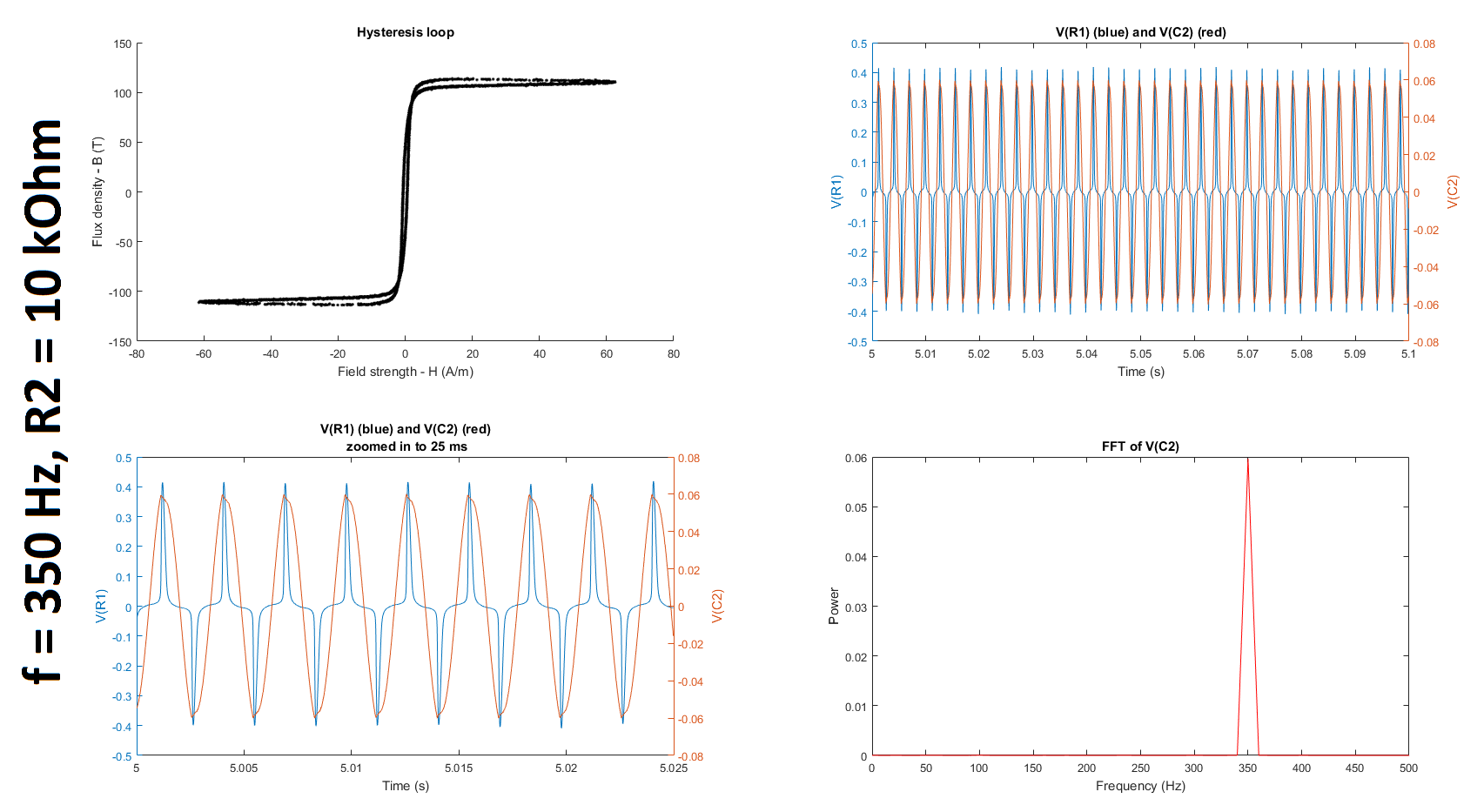
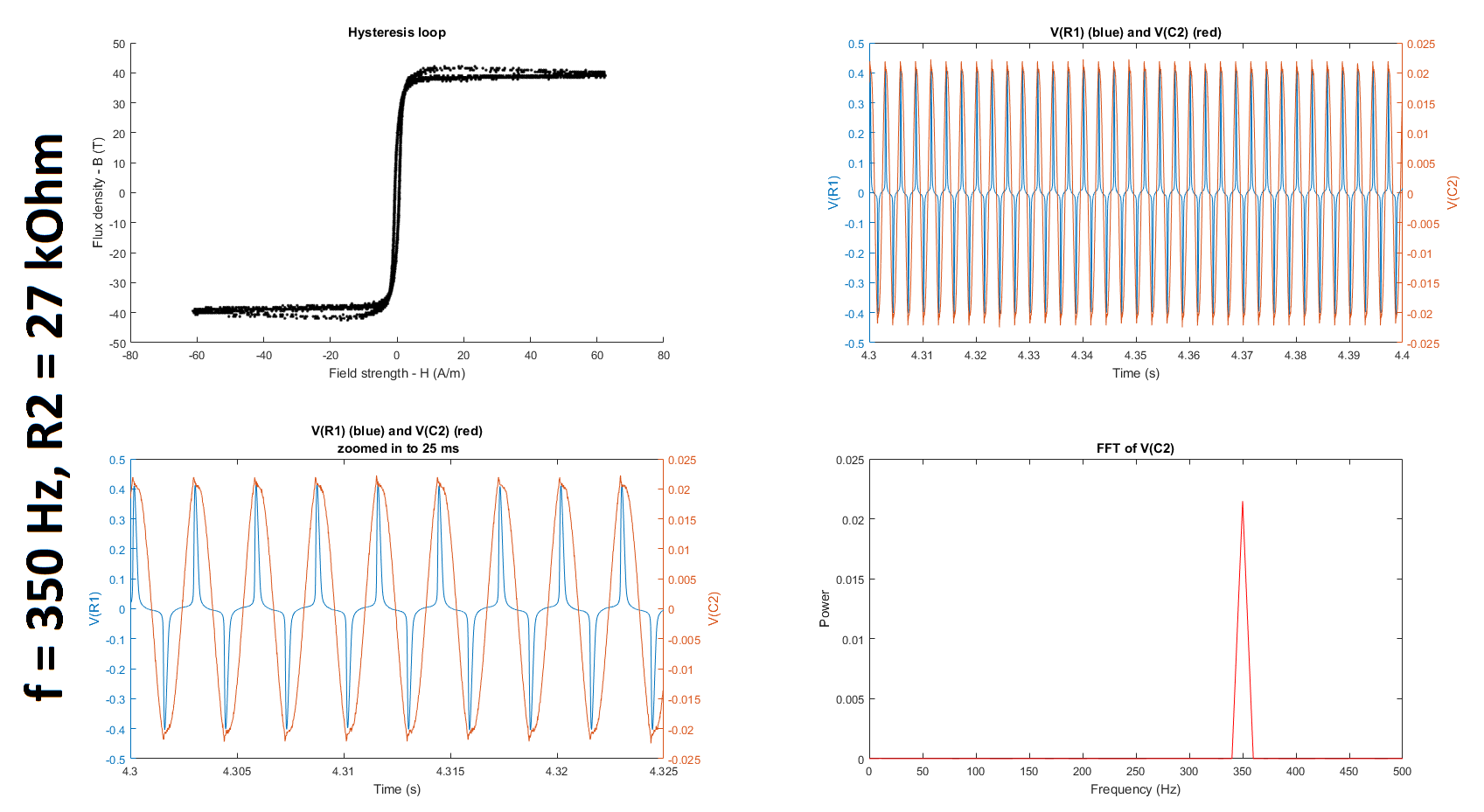
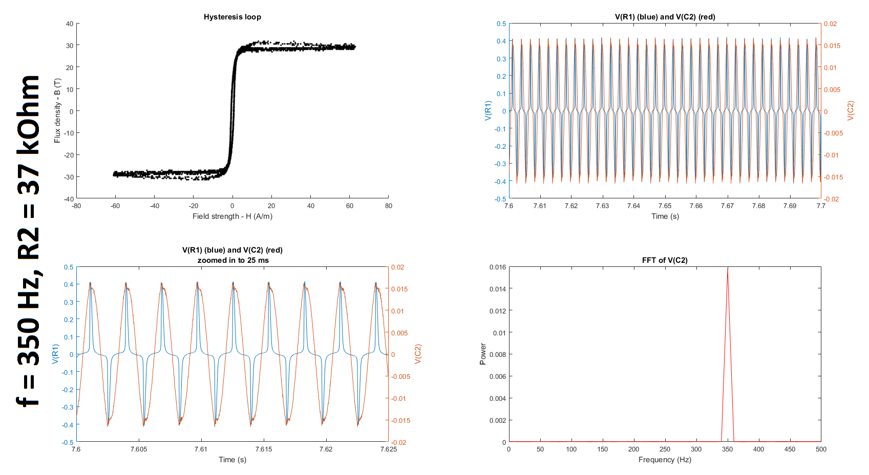
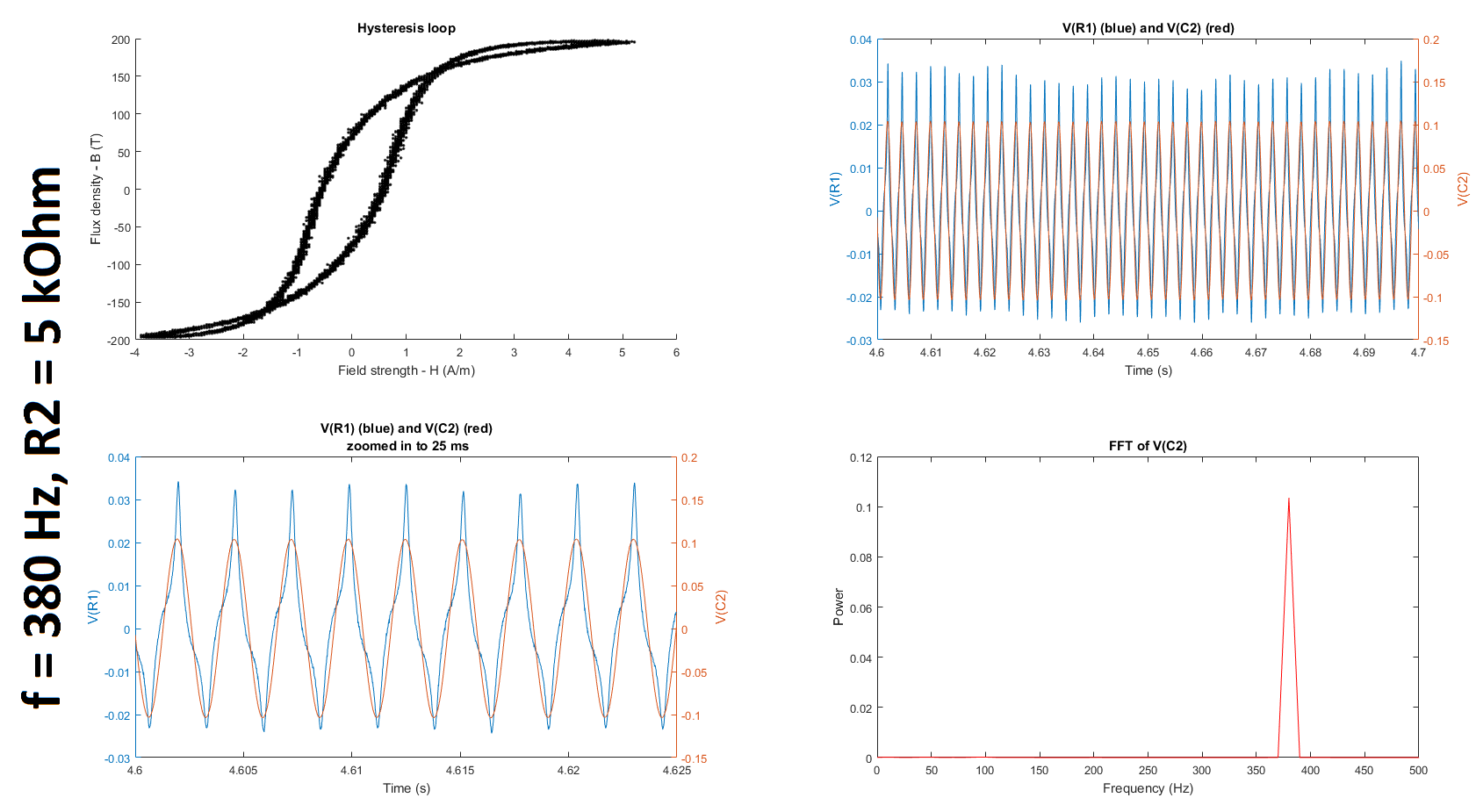
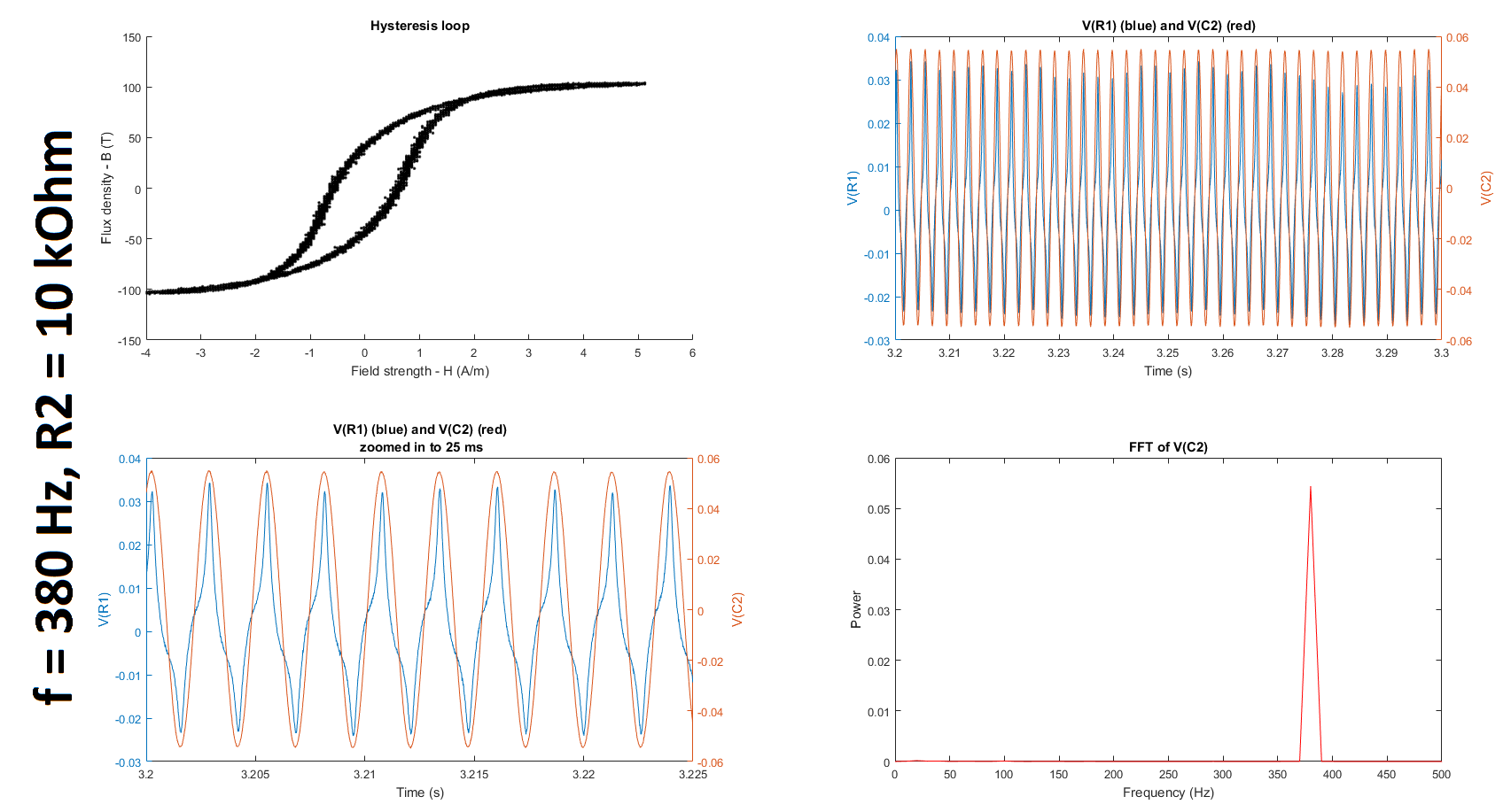
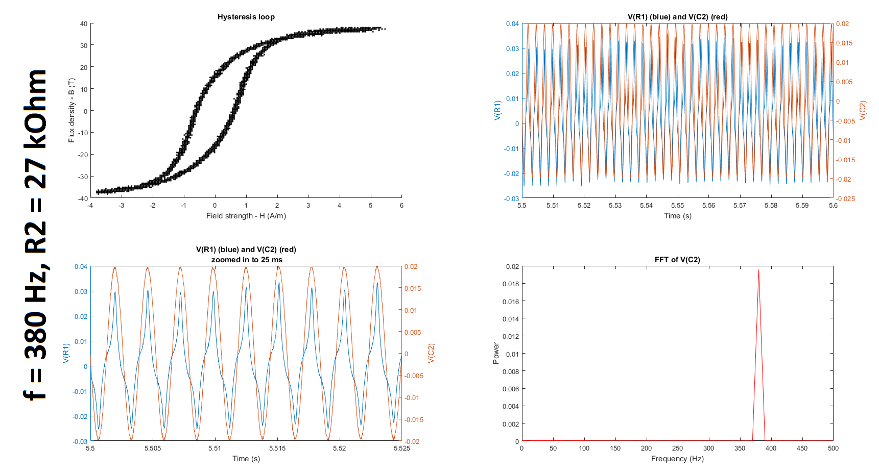
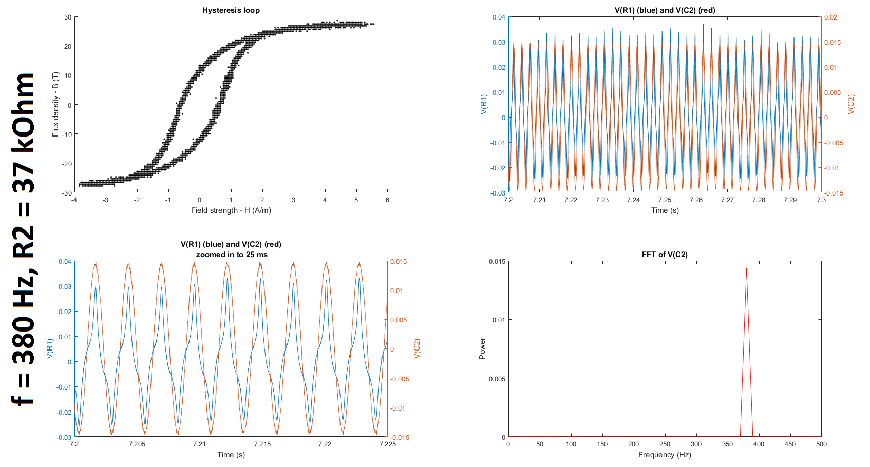
The figures below summarize the results of twelve experiments: \$f = \{50, 350, 380\}\$ Hz \$\times\$ \$R_2 = \{5, 10, 27, 37\}\$ kOhms. Each figure contains four subplots: a hysteresis loop, a plot of the voltage across R1 and the voltage across C2 against time, another plot of the previous but zoomed in, and a plot of the Fourier transform of the voltage across C2.

enter image description here enter image description here enter image description here enter image description here enter image description here enter image description here enter image description here enter image description here enter image description here enter image description here enter image description here enter image description here

Note that to make my hysteresis loop more comparable to those in the datasheets linked above, I converted the raw voltages measured by my probes to magnetic field strength H (units of A/m) and magnetic flux density (units of T) using equations given in the tutorial linked above: $$H \equiv \frac{V_R(t)\cdot N}{R\cdot l_c}$$ where \$V_R\$ is the voltage across the resistor, \$N=6\$ is the number of turns, \$R = 400 \mbox{m}\Omega\$ is the shunt resistor connected to the audio amplifier, and \$l_c = 10.03 \mbox{ cm}\$ is the magnetic path length given here; and $$B(t) \equiv \int_{0}^t{\frac{E(t)}{-N\cdot A_c} dt}$$ where \$E\$ is the electromotive force (EMF) induced in the secondary winding, \$N=6\$ is the number of turns, and \$A_c = 0.88 \mbox{ cm}^2\$ is the cross-sectional area of the core given here. The raw voltages are plotted in the second and third subplots of each figure.

The MATLAB code used to generate H and B from the measurements is shown below:

R = 0.4; % ohms
N = 6; % number of turns
LFe = 10.03E-2; % m
AFe = 8.8E-5; % m^2

H = (V(:, 1)/R)*N/LFe;
B = V(:, 2)/(AFe*N);

figure (1); clf; subplot(2, 2, 1); scatter(H, B, 'k.')
xlabel('Magnetic field strength - H (A/m)')
ylabel('Magnetic flux density - B (T)')

where V(:, 1) and V(:, 2) correspond to the most recent 100 ms of data acquired by the differential probes VM1 and VM2 in the circuit diagram above. I think V(:, 2) already accounts for the integration since it is the voltage across the capacitor on the measurement side, but (Q2-3) I may be missing a multiplication by time in my calculation for B since the units for B are Teslas, which expressed in more fundamental units are \$\frac{V\cdot s}{m^2}\$. It would be great if someone could confirm this / correct me.

The shape of my hysteresis loop looks nowhere that of the hysteresis loop given in either of the datasheets here (page 3) or here even though both report measuring the hysteresis at 50 Hz. (Q2-4) Does anyone why this is the case?

Furthermore, other than H for the 50 Hz input cases, both H and B are orders of magnitude off compared to the values reported in the two datasheets. (Q2-5) Is this something due to the way I'm calculating H and B or due to the circuitry itself? Does this have anything to do with the fact that the integrator has a gain of much less than 1 for the frequencies I'm looking at?

Finally, a question about the way the measurement is being performed: (Q2-6) is it a problem that the integrator on the measurement side is passive? I.e. does the EMF induced in the measurement coil need to be buffered before being fed into the integrator?


Update (8/6/18, 3:15 p.m.): I have divided my question into subquestions posted here (1), here (2), and here (3). Any help would be greatly appreciated.

\$\endgroup\$
4
  • \$\begingroup\$ Your signal source looks suspiciously like 60 Hz ( \$ \omega = 377 \$ ). Your integrator time constant seems wrong. It is a low-pass type filter whose corner frequency should be very much lower than 60 Hz: Increase R2. \$\endgroup\$
    – glen_geek
    Commented Jul 30, 2018 at 16:24
  • \$\begingroup\$ Thanks, @glen_geek. The 377 Hz was just a coincidence. I agree that the cutoff is too low since $$1/(2\pi R_2C_2)$$ = 30 Hz. Don't you mean I should decrease R2? And even then, wouldn't that just affect the gain of the output? \$\endgroup\$ Commented Jul 30, 2018 at 18:05
  • \$\begingroup\$ Certainly affects the gain. Will also affect the B-H hysteresis shape too. I'd make the RC product as large as you can, and still have a decent amplitude on the 'scope Y-axis - perhaps your most sensitive scale is 2mV/cm? The large RC product yields a more accurate integrator. \$\endgroup\$
    – glen_geek
    Commented Jul 31, 2018 at 1:04
  • \$\begingroup\$ @glen_geek, thank you for your comments. I just wanted to point out that \$f = 377\$, not \$\omega\$. I have added results from experiments I performed with a larger R2, as you suggested. Could you please let me know if you have any thoughts on my new questions? \$\endgroup\$ Commented Aug 6, 2018 at 8:15

4 Answers 4

2
\$\begingroup\$

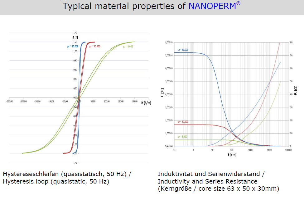
I don't recognize your method but I'm not ruling out that it has some merit but the oscilloscope trace doesn't look right to me. If you want the details of the material used just get hold of the data sheet for the nanoperm material. Extract: -

enter image description here

The hysteresis plot you want is the one in blue I believe.

With 6 turns, the MMF is current applied x 6 turns. To calculate H just divide the MMF by the mean magnetic length of the toroid. That can be calculated as the mean diameter (23 mm) times \$\pi\$ = 0.072 mm.

So if your current is 100 mA, the H field is 0.6/0.072 = 8.3 At/m and this would produce a flux density of about 1 tesla

\$\endgroup\$
11
  • \$\begingroup\$ Thanks for your answer, @Andyaka. Could you please let me know where you got 100 mA from? Also, how did you get the flux density of 1 T? \$\endgroup\$ Commented Aug 6, 2018 at 8:19
  • \$\begingroup\$ Also, I performed the experiments as shown here: meettechniek.info/passive/magnetic-hysteresis.html ("Measuring arrangement with an analog oscilloscope"), except using a passive integrator instead of an active one. \$\endgroup\$ Commented Aug 6, 2018 at 8:25
  • \$\begingroup\$ If you have time, could you please take a look at the updates to my question? After reading through @glen_geek's comments, I noticed a mistake I made in using a single-ended probe instead of a differential one, which I corrected in my update. I also added details about new experiments I performed. The hysteresis loops I'm getting still do not seem to match the manufacturer's results, and I was wondering if you knew why that might be. I have some additional related questions in my update as well. \$\endgroup\$ Commented Aug 6, 2018 at 8:27
  • \$\begingroup\$ "So if your current is 100 mA" i.e. I just guessed at a current to use as an example. May I suggest that you concentrate on one smaller question if you want attention to this. In my opinion you are asking too much to be answered. So raise a new question and get specific about a single test. \$\endgroup\$
    – Andy aka
    Commented Aug 6, 2018 at 10:06
  • 1
    \$\begingroup\$ @VivekSubramanian in your original question you asked: "how can I calculate (Q1-1) the magnetic field strength (in A/m) applied to and (Q1-2) the magnetic flux density (in T) induced in the core". I've given details how you calculate H but, no matter how you try with the experiment you cannot determine flux density without knowing the material permeability. If you can make an experiment to find permeability then that would help. \$\endgroup\$
    – Andy aka
    Commented Aug 7, 2018 at 7:34
2
\$\begingroup\$

I came across a similar question on ResearchGate and found the work done by Mubeen Haadi to be very helpful. Rather than taking a hardware approach to integrating the induced voltage, Haadi took a software approach. I tried Haadi's posted code with some simulated data, and it seemed to work, so I followed in Haadi's footsteps.

I first modified my circuit by placing VM2 directly across terminals of the secondary coil, as shown in the circuit diagram below.

schematic

simulate this circuit – Schematic created using CircuitLab

The voltage induced in the secondary coil is what would have been integrated by the RC integrator (or op-amp integrator). Rather than integrating this voltage with hardware, I integrated the voltage in MATLAB using the cumtrapz function. MATLAB code to generate the hysteresis curve (including the integration) is given here:

% define parameters of setup
R = 400E-3; % ohms
N = 6; % number of turns
LFe = 10.03E-2; % magnetic path legnth, m
AFe = 8.8E-5; % cross-sectional area of core, m^2

% generate time points of integration
t_max = 3; % experiment duration
rate = 80E3; % Fs of AO and AI NIDAQ cards
t = linspace(0, t_max, rate*t_max)';

% meas is the signal recorded by the AI NIDAQ card
VM1 = meas(:, 1);
VM2 = meas(:, 2);

% integrate VM2 and scale it to get the magnetic flux density
dB = VM2/(N*AFe);
B = cumtrapz(t, dB);
B = B - mean(B); % to remove any DC bias

% calculate the current through the primary coil and scale it to get
% magnetic field strength
H = (VM1/R)*N/LFe;

% convert into appropriate units and plot
figure; plot(H*1000/100,B*1000);
xlim([-150 150]); ylim([-1300 1300])
xticks([-140:20:140]); yticks([-1200:200:1200])
grid on
xlabel('H [mA/cm]'); ylabel('B [mT]')

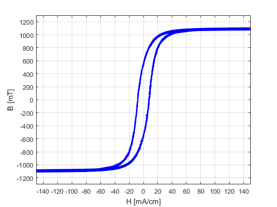
Calculations for H and B were performed according to the tutorial linked here, with the equations given in the update to my question above. (Another useful tutorial linked to me by @laptop2d in one of my subquestions is given here. It contains the same equations for H and B.) The image below shows the hysteresis curve:

enter image description here

This closely matches the curve given in the datasheet 1 (here on page 3) both in terms of appearance and order of magnitude of H and B and resembles the curve in datasheet 2 (here). The loop I measured saturates at about 1.1 T for a field strength of 100 mA/cm while the loop measured by the manufacturer seems to saturate at about 1.2 T for a field strength of 120 mA/cm according to the first datasheet and at 1.2 T for a field strength of 200 mA/cm according to the second datasheet.

I would attribute differences between my curve and the curves shown in the datasheets to differences in the core used by the manufacturer and/or the fact that I'm only using six turns each for the primary and secondary windings, but I'm not really sure. If there are other thoughts as to why there could be differences, I would appreciate the suggestions. Thank you all for your help and contributions.

\$\endgroup\$
0
\$\begingroup\$

Using a big shunt cap load rounds or bulges out your VI plot and gives incorrect results with some low frequency voltage. It makes it impossible to determine what stored energy or Remanence or mutual inductance or primary inductance or eddy current losses you have , which ought to be more important. (Correct me if my assumption is wrong)

I suggest you measure L and losses rather than B or H using a uniform taped winding number of turns.

You can use their tools to calculate saturation where inductance drops 10% rather than measure average BH and count turns and current at 10kHz , 100kHz. https://www.magnetec.de/dimensioning/abacus/abacus.php

Then measure L using an impedance bridge with same inductance in a fixed impedance reference of the same nominal values.

Or if you are lucky , use a vector impedance analyzer

or use an RLC meter with AC coupled meter current and DC coupled external bias if intended for DC use.

Or use an AC only current source with RMS voltage output proportional to L

Or use alternating pulsed current as a flyback inductor measuring V,I,t charge and discharge products with a load .

It depends how you want to use it.

But the ferrite specs with L test results is all I suspect they guarantee at given mA-turns.

If you chose C to resonate in series with 0 phase shift at max current during a sweep, you can measure L and with no C and very low wire/driver ESR measure self capacitance per N turns to get Parallel self Resonant Frequency.

\$\endgroup\$
0
\$\begingroup\$

Q2-4 re: shape of hysteresis loop:
If you take digitized samples of N1 winding current, and use another AtoD channel to take digitized samples of N2 voltage, are these samples simultaneous, or at different times? Any time difference between N1 current sample and integrator voltage sample shows up as modified hysteresis in the B vs. H result. Forcing current at a high rate (high exciting frequency) makes this problem worse.

Current excitation for winding N1 need not be perfectly sinusoidal, but it may help to keep N2's integrator well-behaved. You might increase total series resistance in N1's excitation (along with an increase in excitation voltage) in an attempt to make current more sinusoidal.


Q2-5, Q2-6 re: questions about RC integrator:
The RC integrator is always an approximation at best, but can give a decently accurate result:
\$ V_{C1} = \frac {1}{R_1C_1} \int {V_{N2}(t)} dt \$

provided that \$ V_{N2} >> V_c \$. (where \$ V_{N2} \$ is the 6-turn sense winding voltage.)
Note that the choice of integrator time constant depends on excitation frequency: a 377 Hz source would benefit from a different RC product than a 50 Hz source.

The performance of an RC integrator can be degraded by loading the capacitor with a measuring instrument. For example, an oscilloscope may have a one-Megohm input resistance (plus a very small capacitance in parallel). So the integrator circuit becomes:

schematic

simulate this circuit – Schematic created using CircuitLab
It is best to have R1 << R2. However, this is a compromise, because a large R1 makes for a better integrator (R1xC1 product is large). In the circuit shown above, R1 is close to the geometric mean of capacitive reactance (assuming 377 Hz), and R2's 1M resistance - a reasonable compromise.
R1xC1 product should be large enough to provide an OK integrator for 377 Hz excitation. You could increase C1's capacitance - be aware that this will also reduce the measurement voltage amplitude.

\$\endgroup\$

Your Answer

By clicking “Post Your Answer”, you agree to our terms of service and acknowledge you have read our privacy policy.

Not the answer you're looking for? Browse other questions tagged or ask your own question.