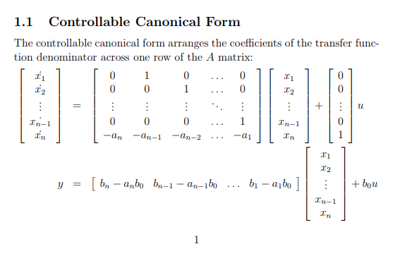
The transformation back, from a state-space model to a transfer function can be done with \$C(sI-A)^{-1}B\$, irrespective of the number of inputs and outputs. In general, you might not end up with a form \$\begin{pmatrix} G(s) & -1 \\ H(s) & 0 \end{pmatrix}\$ though.
The transformation from a transfer function (matrix) to a state-space model is not trivial in case of multiple inputs and multiple outputs. Only the cases with a single input and/or a single output can be solved in general with either the controllable canonical form (requires single input) or the observable canonical form (requires single output).
For example, for a single input two output system
$$
\begin{bmatrix} Y_1(s) \\ Y_2(s)\end{bmatrix}
= \begin{bmatrix} G_1(s) \\ G_2(s)\end{bmatrix} U(s)
$$
you can use the controllable canonical form.
You would first have to put both transfer functions \$G_1(s)\$ and \$G_2(s)\$ on a common denominator and put the obtained denominator coefficients in the matrix \$A\$. The numerator coefficients go in the two rows of the matrix \$C\$. You cannot use the observable canonical form in this case, since then the numerator coefficients would have to go in the matrix \$B\$, but this matrix only has one column, while the numerator coefficients of \$G_1(s)\$ and \$G_2(s)\$ (also after putting them on a common denominator) are in general not equal to each other.
Similarly, for a two input single output case, you cannot use the controllable canonical form (the numerator coefficients of the two transfer functions should go in the matrix \$C\$, but in the single output case, the matrix \$C\$ only has one row). Moreover, the matrix \$B\$ now has two columns, but it should be filled with a bunch of zeros and a row of ones in the last row. This would essentially mean that instead of applying two inputs, you would effectively only have one input equal to the sum of the original two inputs:
$$
B u =
\begin{bmatrix}
0 & 0 \\
\vdots & \vdots \\
0 & 0 \\
1 & 1
\end{bmatrix}
\begin{bmatrix} u_1 \\ u_2 \end{bmatrix}
= \begin{bmatrix}
0 \\
\vdots \\
0 \\
1
\end{bmatrix}
(u_1 + u_2)
$$
I hope this sheds some light on why it is in general impossible to use canoncial forms to transform multiple input multiple output transfer functions into state-space models.
Edit: A possible solution in the multiple input multiple output case is to consider the system as several multiple input single output systems and combine the state-space models of the different subsystems. Afterwards, you can probably apply some kind of model order reduction technique to reduce the number of state variables.
For example, in a two input two output case
$$
\begin{bmatrix} Y_1(s) \\ Y_2(s) \end{bmatrix} =
\begin{bmatrix} G_{11}(s) & G_{12}(s) \\ G_{21}(s) & G_{22}(s) \end{bmatrix}
\begin{bmatrix} U_1(s) \\ U_2(s) \end{bmatrix}
$$
you could consider this as two subsystems, each with two inputs and a single output, and use an observable canonical form for each of them, say
$$
\begin{cases}
\dot{x}_1 = A_1 x_1 + B_1 \begin{bmatrix} u_1 \\ u_2 \end{bmatrix} \\
y_1 = C_1 x_1
\end{cases}
$$
and
$$
\begin{cases}
\dot{x}_2 = A_2 x_2 + B_2 \begin{bmatrix} u_1 \\ u_2 \end{bmatrix} \\
y_2 = C_2 x_2
\end{cases}
$$
Note that \$x_1\$ and \$x_2\$ are state vectors here, not just the first and the second element of a state vector \$x\$.
Next, you can combine the two state-space submodels:
$$
\begin{cases}
\begin{bmatrix} \dot{x}_1 \\ \dot{x}_2 \end{bmatrix} =
\begin{bmatrix} A_1 & 0 \\ 0 & A_2 \end{bmatrix}
\begin{bmatrix} x_1 \\ x_2 \end{bmatrix} +
\begin{bmatrix} B_1 \\ B_2 \end{bmatrix}
\begin{bmatrix} u_1 \\ u_2 \end{bmatrix} \\
\begin{bmatrix} y_1 \\ y_2 \end{bmatrix} =
\begin{bmatrix} C_1 & 0 \\ 0 & C_2 \end{bmatrix}
\begin{bmatrix} x_1 \\ x_2 \end{bmatrix}
\end{cases}
$$
and like this obtain a state-space model of the two input two output system.

