Why does tracking different plant states result in totally different observer estimates?

Question

I am trying to design a Luenberger observer (or a full state feedback observer) such that with one sensor available I can estimate all the states. A good tutorial is shown here.

My system is 4th order:

num = [-0.00198 2];
den = [1 0.1201 12.22 0.4201 2];
sys = tf(num,den);
[A, B, C, D] = tf2ss(num,den);

First I have a row vector of poles to get my desired response:

poles = [-2.6 + 1i*2.39, -2.6 - 1i*2.39, -100, -120];
K = acker(A,B,poles)
rank(obsv(A,C));  % =4
Mo = rank([C;C*A;C*A^2;C*A^3]) % =4

I then proceed to calculate the plant poles and thus the poles I want for my observer should be around 3x faster.

plant = (A-B*K);
poles_cl = eig(plant)

poles = 3*poles_cl  % THIS IS WRONG
des_poles = (min(real(poles_cl))*3)-(1:4); %This is better

des_poles =

 -361.0000 -362.0000 -363.0000 -364.0000

I then proceed to use Ackermann's formula for pole placement using the new poles:

% design observer by placing poles of A-LC at des_poles 
L=acker(A',C',poles_des)'
eig_obs = eig(A-L*C) 

L =

   1.0e+09 *

    8.6121
    0.1037
    0.0005
    0.0000

eig_obs =

 -361.0000
 -362.0000
 -363.0000
 -364.0000

And finally plot. For the observer (software) to give us all the states as output we need to set C = eye(4):

C = eye(4);
mysys=ss(A-L*C,[B L],C,0); %Not sure if this is correct
tf(mysys)
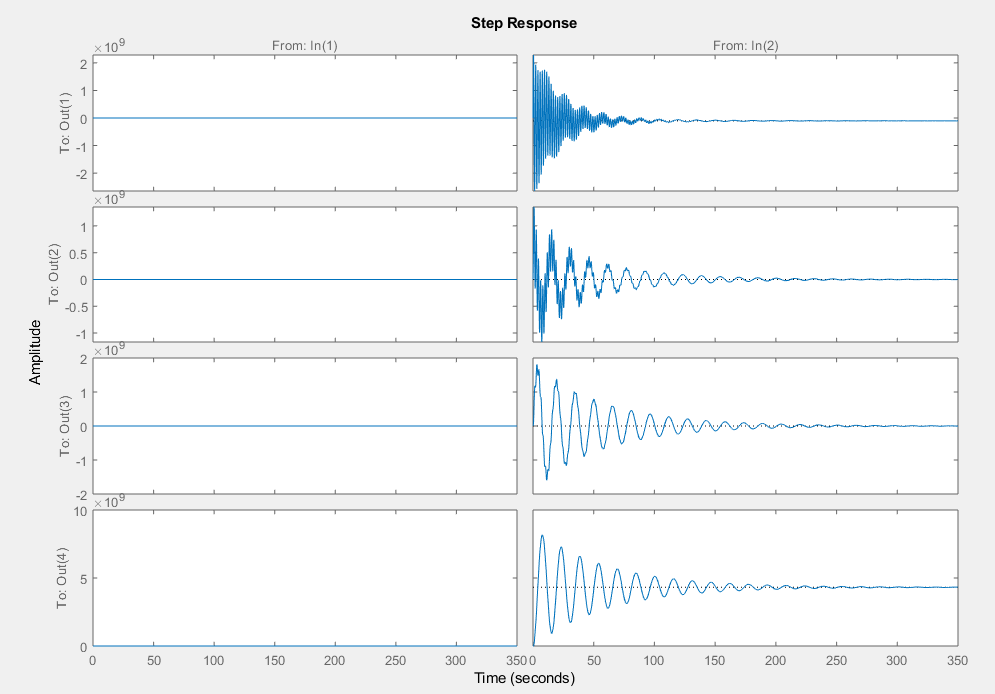
step(mysys)

Four outputs can be seen:

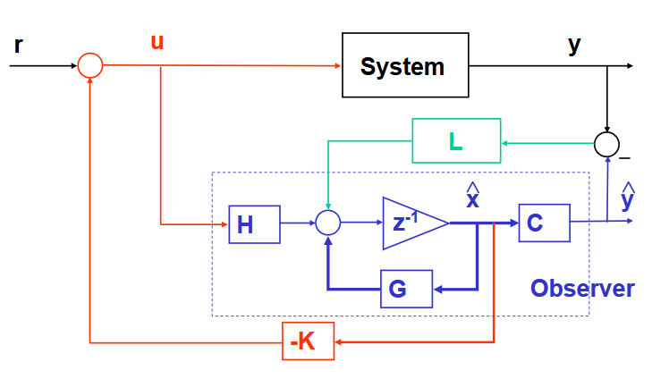
Following this model for a full state feedback observer:

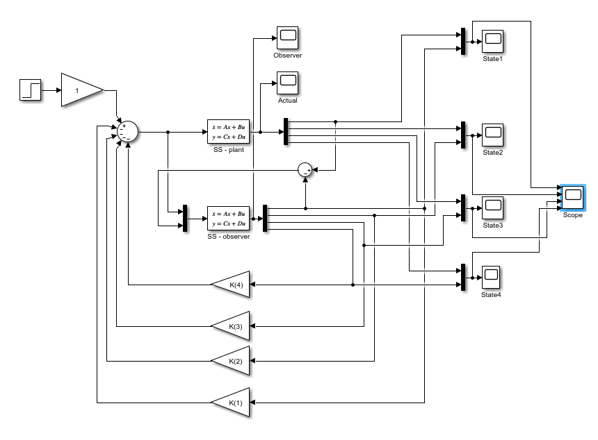
I am then trying to verify the results on Simulink and am having issue with the block diagram. As can be seen I have two state space models, one for the real plant and one for the observer.

In the below diagram I am comparing state 1, which results in the second graph depicted below.

I am using the base workspace generated by the code above:

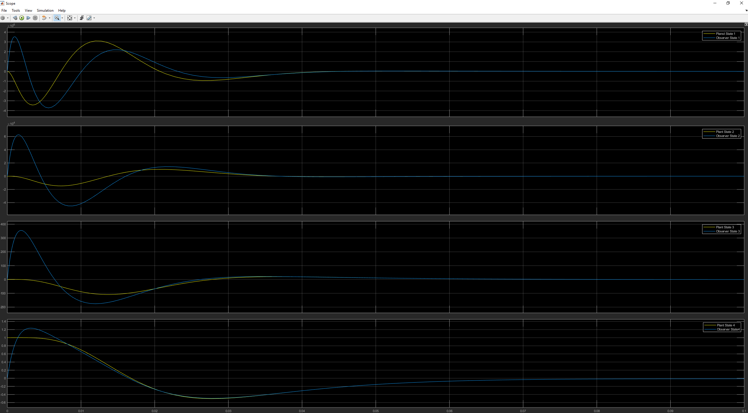
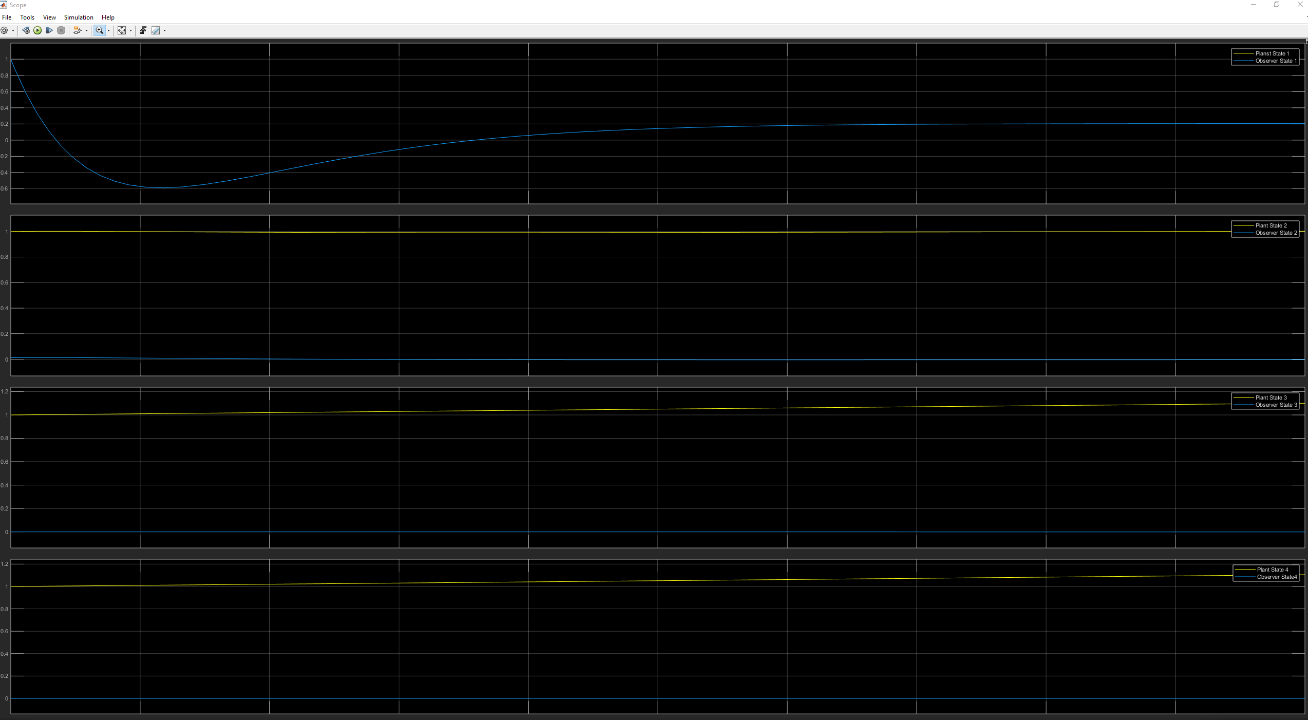
Upon running I get an output from the observer which does not track or follow the plant as expected:

Actual and Observer states when comparing state 4 through summing block:

Actual and Observer states when comparing state 1 through summing block:

Any suggestions on why the state I choose to compare via the summing block is effecting the observer estimations would be appreciated.

---

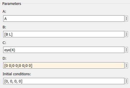
Observer Parameters:

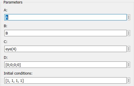
Plant Parameters:

1. Why does the state which I am comparing, effect the observer response?

Answer 1

This answer pertains to the question title "How to design an observer to estimate all states from a single sensor".

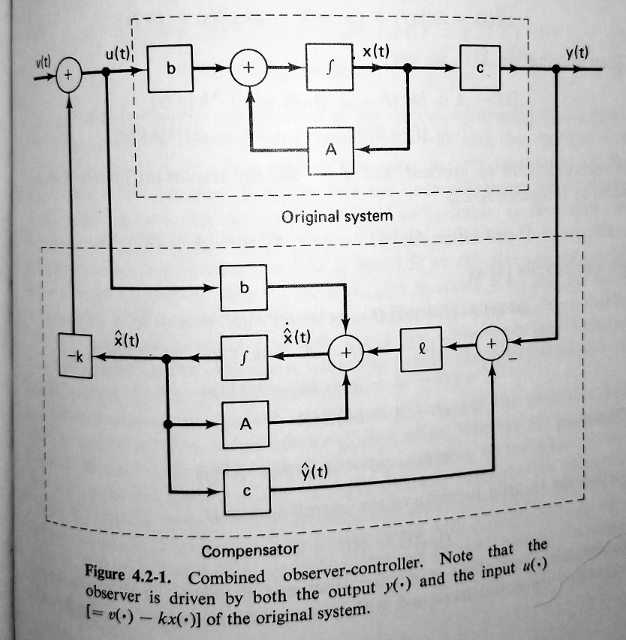
I'm pretty sure that you have the input vector to the compensator reversed. You either need to reverse the order that signals go into the multiplexer, or you need to reverse the order of the B matrix in the compensator (by changing it to [L B]. For reference here's a picture.

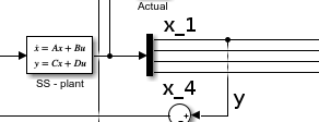
By picking off the \$x_1\$ term from your state vector you are also effectively using \$C=\left[\matrix{1 & 0 & 0 & 0}\right]\$. See the picture. I suspect, but do not know, that the tf2ss function returns C=[0 0 0 1], you should check this.

Note that Simulink will let you draw out the compensator pretty much the way it's done here -- it'll accept matrix gains and carry vector signals, and IIRC integrate vectors. So you can have a complete block diagram of what you want, instead of trying to get all the graphical 'i's and 't's dotted to match the textual specification in the definition block.

From Linear Systems, Kailath, Prentice-Hall, 1980.

Answer 2

This answer pertains to the current title ("Why Does Tracking Different Plant States Result In Totally Different Observer Estimates").

The answer is -- turn off Matlab until you know what you're doing, and then do the math. The answer should be clear. If it's not, do the math some more.

The observer equations (from the picture in my first answer) are $$ \frac{d\hat{x}}{dt} = A \hat{x} + B u + L\left(y - \hat{y}\right), \hat{y} = C \hat{x}$$

Using simple linear algebra, you can eliminate the reference to \$\hat{y}\$ in the first equation:$$ \frac{d\hat{x}}{dt} = \left(A - LC\right) \hat{x} + \left[\matrix{B & L}\right] \left[\matrix{u \\ y}\right], \hat{y} = C \hat{x}$$

The phrase "Tracking different plant states" translates, mathematically, to "changing the value of \$C\$". Looking at the second equation above, it's pretty obvious that if \$A - LC_1 \ne A - LC_2\$, then the two systems are going to act differently. It's really that simple.