How to find gain and phase crossover from a Nyquist plot?

Question

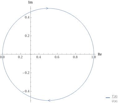
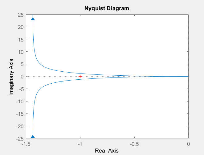
Note: I need to do this by hand which is why I'm struggling. I'm only using MATLAB here to show the nyquist plot, and I was also using it to try and check my answer.

Edit: There are poles at -50, -10 and 0. So none on the RHS but 1 on the axis. I know this implies marginally stable, but I need to provide an explanation based on the Nyquist plot and I thought using crossovers and margins would be the best way to achieve this. (Since the pole explanation is easy to obtain just by looking at the trasfer function and doesn't relate to the Nyquist)

Using this Nyquist plot, I need to determine the stability of the system. I know that I can do this by comparing the phase and gain crossover frequencies, and gain and phase margins. The margins are calculated using the frequencies, so I need to find them to carry on.

• Phase crossover is the frequency when the plot crosses the negative real axis
• Gain crossover is the frequency when magnitude is 1

I need to be able to do this by referring to the Nyquist plot, but I'm not sure how to do this. MATLAB doesn't provide any frequency data at the crossover points as it only shows certain data when using the data tips, so how could I estimate the frequencies?

Answer 1

To use Matlab for checking the answer which was calculated by hand, try one of the below methods,

1. allmargin(system)
2. increase number of frequency points in the Nyquist plot by manually supplying a large number of frequency points. e.g. nyquist(system, [0:1e-2:1e3]). and then use the cursor. Newer versions of Matlab will show the frequency as well as other details from which you can manually calculate the margins
3. Use the option given in the context menu / right click menu to show the margins using the cursor / data label.

Example from Mathworks

Sample image from mathworks

Note: Remember that, to calculate margins, you plot the Nyquist for the open loop system and that too where the final system is transformed into a unity feedback configuration.

Note : To calculate by hand, use the conditions \$|G(s)| = 1\$ and \$\angle G(s) = \pi\$ to solve for the gain cross over and phase cross over frequency(ies) respectively. Here \$G(s)\$ is the open loop transfer function of the unity feedback system. _{Information needed for this is not given in the question.}

Answer 2

A Nyquist plot will not allow one to find the gain crossover frequency or the phase crossover frequency, unless these frequencies are added to the plot. The curve itself does not contain any frequency information. Indeed, two different transfer functions can have the same Nyquist plot. For example, all transfer functions of the form

$$\frac{1}{1+\frac{s}{k}}$$

(where k is any positive number)

have the same Nyquist plot, namely

Although we cannot find the gain or phase crossover frequencies from an unadorned Nyquist plot alone, we can, however, find the gain and phase margins.

"The" gain margin is the dB gain where the phase is some odd multiple of \$180^{\circ}\$. (I put "the" in parentheses because there may be more than one frequency where the phase is an odd multiple of \$180^{\circ}\$.) On a Nyquist plot, points with such a phase are points on the negative real axis.

"The" phase margin is the difference between the phase where the gain is 0 dB, and \$180^{\circ}\$. (I put "the" in parentheses because there may be more than one frequency where the dB gain is 0.) On a Nyquist plot, unity gain points lie on a unit circle.

Looking at the Nyquist plot in the question we see that the gain at the point where the Nyquist curve crosses the negative real axis is perhaps 0 i.e. -\$\infty\$ dB. It isn't exactly clear, but it appears to be certainly less than unity gain (i.e. 0 dB). The point where the lower arm of the Nyquist plot crosses the unit circle is just a few degrees (if that). So the phase margin is only a few degrees. Finally, the Nyquist plot does not encircle the point -1+j0, so the transfer function is stable.