Overview
Note: I've added some Glowscript/VPython code to help illustrate the value of using software programming tools. We have so much available to us, provided by many contributors to whom we owe much. Learn well to use the gifts we've been handed by these wonderful people.
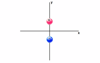
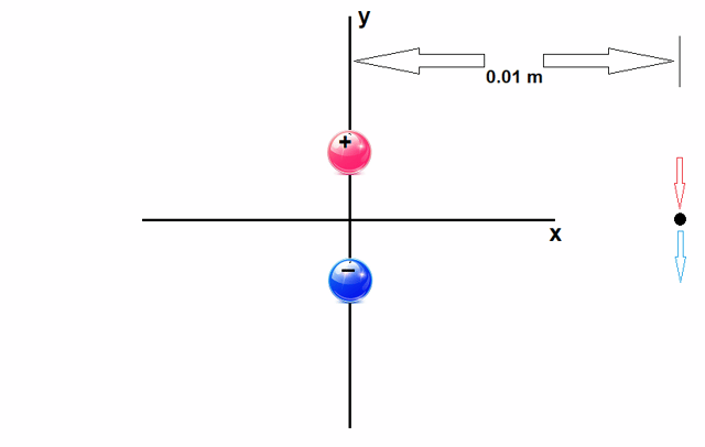
Here is what I imagine for the dipole of \$\left(1\times10^{-15}\: C\!\cdot\! m\right)\hat{y}\$. (This might be \$3\frac13\:\text{pC}\$ separated by \$300\:\mu\text{m}\$ to represent your dipole moment, for example.)

(I drew that with Microsoft Paint.)
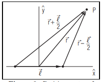
The field at any point around the above dipole will be the superposition (sum) of the effects of both charges. So:
$$\begin{align*}
\vec{E}&=\vec{E}_++\vec{E}_-\\\\&=\frac1{4\pi\epsilon_{_0}}\frac{q_+}{\mid\vec{r}_+\mid^2}\hat{r}_+ + \frac1{4\pi\epsilon_{_0}}\frac{q_-}{\mid\vec{r}_-\mid^2}\hat{r}_-\\\\&=k_e\left[\frac{q_+}{\mid\vec{r}_+\mid^2}\hat{r}_+ + \frac{q_-}{\mid\vec{r}_-\mid^2}\hat{r}_-\right], \text{where }k_e=\frac1{4\pi\epsilon_{_0}}\approx 9\times10^9\:\frac{N\cdot m^2}{C^2}
\end{align*}$$
(More exactly, \$k_e\approx 8.98755179\times10^9\:\frac{N\cdot m^2}{C^2}\$)
It's pretty simple.
Python -- Learn to Use It
Before I dig into your specific questions, this is a good place to make a case for learning to use Python. It's just too handy to ignore.
Let's express the above knowledge in VPython (I'll be using GlowScript 3.1 VPython):
ke = 8.98755179e9   # eqivalent for 1/(4*pi*e0) in SI units.

# Dipole charge and separation.
q = 5e-12 / 1.5     # 3 1/3 pC
s = 300e-6          # 300 microns

# Dipole moment.
p = q * s

# Computes E-field for a charge, as seen from any given point around it.
def E( qm, qp ) : return def ( p ) : return ke * qm * norm(p-qp) / mag(p-qp)**2

# E-field functions for the positive and negative charges.
ep = E(  q, vector( 0,  s/2, 0 ) )
en = E( -q, vector( 0, -s/2, 0 ) )

print( "Dipole moment: ", p, "C m")
That prints out:
Dipole moment: 1e-15 C m
I added a little extra code above because I'll be using this code, later, and will need the extra bits then. You can check this out on your own by using this link.
Case (a)
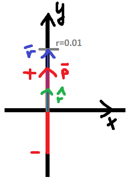
I'd draw it up this way:

At a point \$10\:\text{cm}\$ along the positive x-axis, the magnitudes due to the two charges along \$\hat{x}\$ cancel out, leaving only that caused along \$\hat{y}\$, as shown above in the image. These residuals (are shown in their associated color and direction and they) will add together and point downward, according to the usual conventions. So pointing as \$-\hat{y}\$, or \$\langle 0,-1,0\rangle\$. That's my qualitative expectation.
\$\vec{r}_+=\langle x, 0, 0\rangle-\langle 0, \frac{s}2, 0\rangle=\langle x,-\frac{s}{2},0\rangle\$ and \$\vec{r}_-=\langle x, 0, 0\rangle-\langle 0, -\frac{s}2, 0\rangle=\langle x,\frac{s}{2},0\rangle\$.
\$\hat{r}_+=\frac{\vec{r}_+}{\mid \vec{r}_+\mid}=\frac{\langle x,\,-\frac{s}{2},\,0\rangle}{\sqrt{x^2+\left(-\frac{s}2\right)^2}}=\frac{\langle x,\,-\frac{s}{2},\,0\rangle}{\sqrt{x^2+\left(\frac{s}2\right)^2}}\$ and \$\hat{r}_-=\frac{\vec{r}_-}{\mid \vec{r}_-\mid}=\frac{\langle x,\,\frac{s}{2},\,0\rangle}{\sqrt{x^2+\left(\frac{s}2\right)^2}}\$.
Let's now prove a result:
$$\begin{align*}
\vec{E}_\bot&=\vec{E}_++\vec{E}_-
\\\\
&=\frac1{4\pi\epsilon_{_0}}\cdot\frac{q}{\left[x^2+\left(\frac{s}2\right)^2\right]}\cdot\frac{\langle x,-\frac{s}2,0\rangle}{\sqrt{x^2+\left(\frac{s}2\right)^2}} + \frac1{4\pi\epsilon_{_0}}\cdot\frac{-q}{\left[x^2+\left(\frac{s}2\right)^2\right]}\cdot\frac{\langle x,\frac{s}2,0\rangle}{\sqrt{x^2+\left(\frac{s}2\right)^2}}
\\\\
&=\frac1{4\pi\epsilon_{_0}}\cdot\frac{q}{\left[x^2+\left(\frac{s}2\right)^2\right]^\frac32}\cdot\langle x-x,-\frac{s}2-\frac{s}2,0-0\rangle
\\\\
&=\frac1{4\pi\epsilon_{_0}}\cdot\frac{q}{\left[x^2+\left(\frac{s}2\right)^2\right]^\frac32}\cdot\langle 0,-s,0\rangle
\\\\
&=\frac1{4\pi\epsilon_{_0}}\cdot\frac{q s}{\left[x^2+\left(\frac{s}2\right)^2\right]^\frac32}\cdot\langle 0,-1,0\rangle
\end{align*}$$
There is no information given about the separation \$s\$ of the charges. Only the dipole moment of \$p=q s\$ is given. So, the dipole approximation with \$r=x=10\:\text{cm}\$ leaves you only with:
$$\begin{align*}
\mid \vec{E}_\bot\mid&=\left[\frac1{4\pi\epsilon_{_0}}\right]\cdot\frac{q s}{x^3}=\left[9\times10^9\frac{N\cdot m^2}{C^2}\right]\cdot \frac{p}{r^3}
\end{align*}$$
And you computed the result correctly as \$9\:\frac{N}{C}\langle 0,-1,0\rangle\$ or \$-9\:\frac{N}{C}\langle 0,1,0\rangle\$.
Let's check back in with that GlowScript, again. Adding the following code:
# Magnitude of distance from dipole.
r = 10e-3         # 1 cm

# Perpendicular position:
pp = r * vector( 1, 0, 0 )

# Net field.
eppnet = ep( pp ) + en( pp )

print( "Perpendicular: ", mag( eppnet ), "N/C", norm( eppnet ) )
We now get:
Dipole moment:  1e-15 C m
Perpendicular:  8.98452 N/C < 0, -1, 0 >
Not bad. Easy to use and understand, too.
Case (b)
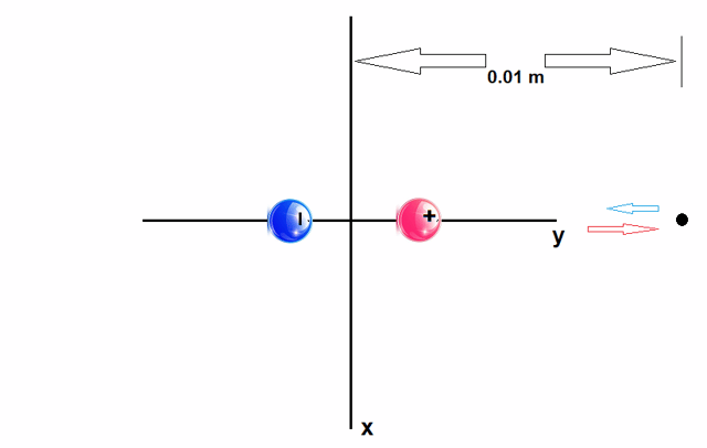
I'd draw it up this way:

At a point \$10\:\text{cm}\$ along the positive y-axis, the magnitudes due to the two charges along \$\hat{x}\$ are zero and those along \$\hat{y}\$ are shown in the image. (One is larger in magnitude than the other.)
\$\vec{r}_+=\langle 0, y, 0\rangle-\langle 0, \frac{s}2, 0\rangle=\langle 0,y-\frac{s}{2},0\rangle\$ and \$\vec{r}_-=\langle 0, y, 0\rangle-\langle 0, -\frac{s}2, 0\rangle=\langle 0,y+\frac{s}{2},0\rangle\$.
\$\hat{r}_+=\frac{\vec{r}_+}{\mid \vec{r}_+\mid}=\frac{\langle 0,\,y-\frac{s}{2},\,0\rangle}{\sqrt{0^2+\left(y-\frac{s}{2}\right)^2}}=\langle 0,\,1,\,0\rangle\$ and \$\hat{r}_-=\frac{\vec{r}_-}{\mid \vec{r}_-\mid}=\frac{\langle 0,\,y+\frac{s}{2},\,0\rangle}{\sqrt{0^2+\left(y+\frac{s}{2}\right)^2}}=\langle 0,\,1,\,0\rangle\$.
Let's again prove a result:
$$\begin{align*}
\vec{E}_\text{on axis}&=\vec{E}_++\vec{E}_-
\\\\
&=\frac1{4\pi\epsilon_{_0}}\cdot\frac{q}{\left[\left(y-\frac{s}2\right)^2\right]}\cdot\langle 0,1,0\rangle + \frac1{4\pi\epsilon_{_0}}\cdot\frac{-q}{\left[\left(y+\frac{s}2\right)^2\right]}\cdot\langle 0,1,0\rangle
\\\\
&=\frac1{4\pi\epsilon_{_0}}\cdot q\left[\frac{1}{\left[\left(y-\frac{s}2\right)^2\right]} + \frac{-1}{\left[\left(y+\frac{s}2\right)^2\right]}\right]\cdot\langle 0,1,0\rangle
\\\\
&=\frac1{4\pi\epsilon_{_0}}\cdot q\left[\frac{\left(y+\frac{s}2\right)^2-\left(y-\frac{s}2\right)^2}{\left[\left(y-\frac{s}2\right)^2\right]\left[\left(y+\frac{s}2\right)^2\right]}\right]\cdot\langle 0,1,0\rangle
\\\\
&=\frac1{4\pi\epsilon_{_0}}\cdot\left[\frac{2 q s y}{\left[\left(y-\frac{s}2\right)^2\right]\left[\left(y+\frac{s}2\right)^2\right]}\right]\cdot\langle 0,1,0\rangle
\end{align*}$$
Again, there is no information given about the separation \$s\$ of the charges. Only the dipole moment of \$p=q s\$ is given. So, the dipole approximation with \$r=y=10\:\text{cm}\$ leaves you only with:
$$\begin{align*}
\mid \vec{E}_\text{on axis}\mid&=\left[\frac1{4\pi\epsilon_{_0}}\right]\cdot\frac{2 q s y}{y^4}=\left[9\times10^9\frac{N\cdot m^2}{C^2}\right]\cdot \frac{2 p}{r^3}
\end{align*}$$
Which should be twice as large, in magnitude, as for case (a).
But in this case the sign is positive.
Let's check back in with GlowScript. Adding the following code:
# On-axis position.
onaxisp = r * vector( 0, 1, 0 )

# Net field, again.
eonaxisnet = ep( onaxisp ) + en( onaxisp )

print( "On axis: ", mag( eonaxisnet ), "N/C", norm( eonaxisnet )
We now get:
Dipole moment:  1e-15 C m
Perpendicular:  8.98452 N/C < 0, -1, 0 >
On axis:  17.9832 N/C < 0, 1, 0 >
Again, not bad.
Case (e)
I thought I'd add a little bit towards this case:
$$
\begin{align*}
\begin{array}{rl}
{\vec{r}_+} &= \vphantom{\langle \frac{r}{\sqrt{2}}, \frac{r}{\sqrt{2}}, 0\rangle-\langle 0, \frac{s}2, 0\rangle}\\\\
&= \vphantom{\langle \frac{r}{\sqrt{2}},\frac{r}{\sqrt{2}}-\frac{s}{2},0\rangle}\\\\
{\hat{r}_+} &= \vphantom{\frac{\vec{r}_+}{\mid \vec{r}_+\mid}}\\\\
&= \vphantom{\frac{\langle \frac{r}{\sqrt{2}},\frac{r}{\sqrt{2}}-\frac{s}{2},0\rangle}{\sqrt{\left(\frac{r}{\sqrt{2}}\right)^2+\left(\frac{r}{\sqrt{2}}-\frac{s}{2}\right)^2}}}
\end{array}
&&
{
\begin{array}{l}
\langle \frac{r}{\sqrt{2}}, \frac{r}{\sqrt{2}}, 0\rangle-\langle 0, \frac{s}2, 0\rangle\\\\
\langle \frac{r}{\sqrt{2}},\frac{r}{\sqrt{2}}-\frac{s}{2},0\rangle\\\\
\frac{\vec{r}_+}{\mid \vec{r}_+\mid}\\\\
\frac{\langle \frac{r}{\sqrt{2}},\frac{r}{\sqrt{2}}-\frac{s}{2},0\rangle}{\sqrt{\left(\frac{r}{\sqrt{2}}\right)^2+\left(\frac{r}{\sqrt{2}}-\frac{s}{2}\right)^2}}
\end{array}
}
&&&&
\begin{array}{rl}
{\vec{r}_-} &= \vphantom{\langle \frac{r}{\sqrt{2}}, \frac{r}{\sqrt{2}}, 0\rangle-\langle 0, -\frac{s}2, 0\rangle}\\\\
&= \vphantom{\langle \frac{r}{\sqrt{2}},\frac{r}{\sqrt{2}}+\frac{s}{2},0\rangle}\\\\
{\hat{r}_-} &= \vphantom{\frac{\vec{r}_-}{\mid \vec{r}_-\mid}}\\\\
&= \vphantom{\frac{\langle \frac{r}{\sqrt{2}},\frac{r}{\sqrt{2}}+\frac{s}{2},0\rangle}{\sqrt{\left(\frac{r}{\sqrt{2}}\right)^2+\left(\frac{r}{\sqrt{2}}+\frac{s}{2}\right)^2}}}
\end{array}
&
{
\begin{array}{l}
\langle \frac{r}{\sqrt{2}}, \frac{r}{\sqrt{2}}, 0\rangle-\langle 0, -\frac{s}2, 0\rangle\\\\
\langle \frac{r}{\sqrt{2}},\frac{r}{\sqrt{2}}+\frac{s}{2},0\rangle\\\\
\frac{\vec{r}_-}{\mid \vec{r}_-\mid}\\\\
\frac{\langle \frac{r}{\sqrt{2}},\frac{r}{\sqrt{2}}+\frac{s}{2},0\rangle}{\sqrt{\left(\frac{r}{\sqrt{2}}\right)^2+\left(\frac{r}{\sqrt{2}}+\frac{s}{2}\right)^2}}
\end{array}
}
\end{align*}
$$
Once again,
$$\begin{align*}
\vec{E}_{45^\circ}&=\vec{E}_++\vec{E}_-=\frac1{4\pi\epsilon_{_0}}\frac{q_+}{\mid\vec{r}_+\mid^2}\hat{r}_+ + \frac1{4\pi\epsilon_{_0}}\frac{q_-}{\mid\vec{r}_-\mid^2}\hat{r}_-
\end{align*}$$
If you follow through, you may also find (for \$r\gg s\$): \$\vec{E}_{45^\circ}=\left[\frac1{4\pi\epsilon_{_0}}\right]\cdot \frac{p}{r^3}\cdot\langle \frac32,\frac12,0\rangle\$. So I get \$\approx 14.23\:\frac{N}{C}\:\angle 18.435^\circ\$.
Returning to Glowscript and adding this code:
# 45-degree, quadrant 1 position.
ap = r * vector( cos( pi/4 ), sin( pi/4 ), 0 )

# Net field, yet again.
eanet = ep( ap ) + en( ap )

print( "45 degree: ", mag( eanet ), "N/C", norm( eanet ) )
I get:
Dipole moment:  1e-15 C m
Perpendicular:  8.98452 N/C < 0, -1, 0 >
On axis:  17.9832 N/C < 0, 1, 0 >
45 degree:  14.2107 N/C < 0.948762, 0.315993, 0 >
(Note that it computes a normal that has a hypotenuse of 1. I had to do that, too. But didn't want to write the expression that way, preferring to use an unnormalized vector, instead. The magnitude results are the same, either way.)
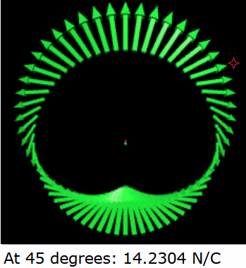
I also did a quick visual simulation using Glowscript (see code here, for example.) Using \$3\frac13\:\text{pC}\$, separated by \$300\:\mu\text{m}\$, made the dipole pretty small in the image:

(That result was achieved using \$9\times 10^9\$ rounded figure and not the more exact figure used in earlier simulations.)
But it gets the point across. I also performed a computation using Python and displayed the value at the bottom. (The arrow with the little red 'star' at its tip is this vector at \$45^\circ\$.) Matches with my expectations, above.
Summary
That's as far as I want to go, here. I feel it is sufficient to show how to reach case (b) and that you should be able to translate the above into the context of your own book (which I do not have), in order to produce the remaining results.
Finally, with VPython, the above could have been done slightly differently:
ke = 8.98755179e9   # eqivalent for 1/(4*pi*e0) in SI units.

class StaticCharge:
  def __init__( self, charge, position ):
    self.charge = charge
    self.position = position
  def q( self ) : return self.charge
  def pos( self ) : return self.position
  # Coulomb’s law (stationary charges -- breaks down in relativistic cases.)
  def E( self, pos ) : return ke * self.charge / mag2(pos-self.position) * hat(pos-self.position)

class Dipole:
  def __init__( self, charge, separation, axis ):
    self.charge = charge
    self.axis = axis
    self.separation = separation
    self.moment = charge * separation
    self.positive = StaticCharge( charge, separation/2 * axis )
    self.negative = StaticCharge( -charge, -separation/2 * axis )
  def posp( self ) : return self.positive.pos()
  def posn( self ) : return self.negative.pos()
  def sep( self ) : return self.separation
  def p( self ) : return self.moment
  def E( self, pos ) : return self.positive.E( pos ) + self.negative.E( pos )
  def D( self, pos ) :
    efield = self.E( pos )
    return f"{mag( efield )} N/C {hat( efield )}"


# Input: dipole moment and charge.
p = 1e-15           # dipole momentum
q = 10e-12 / 3      # 3 1/3 pC

# Input: radial distance.
r = 10e-3           # 1 cm

# My dipole: has charge q, separation p/q, and aligned on the y-axis.
mydipole = Dipole( q, p/q, vector( 0, 1, 0 ) )

# Three points of interest around the dipole.
perpendicular = r * vector( 1, 0, 0 )
onaxis = r * vector( 0, 1, 0 )
fortyfive = r * vector( cos( pi/4 ), sin( pi/4 ), 0 )

# Display the E-field at these three points around the dipole.
print( "Perpendicular: ", mydipole.D( perpendicular ) )
print( "On axis: ", mydipole.D( onaxis ) )
print( "45 degrees: ", mydipole.D( fortyfive ) )

# Create graphical balls for the dipole.
ballp = sphere( pos = mydipole.posp(), radius = mydipole.sep()/2, color = color.red )
balln = sphere( pos = mydipole.posn(), radius = -mydipole.sep()/2, color = color.cyan )

# Perform a loop generating 64 vectors in a circle around the dipole.
N = 64
theta = 0
dtheta = 2*pi / N
while theta < 2*pi:
  ro = r * vector( cos(theta), sin(theta), 0 )
  arrow( pos = ro, axis = 2e-4*mydipole.E( ro ), color = color.green )
  theta = theta + dtheta
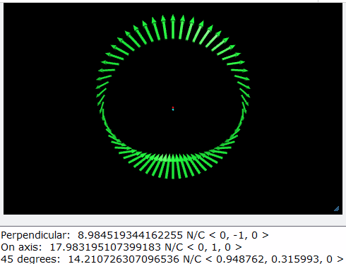
For the above code see here. This outputs:

Pretty nice and easy.
An Added Diversion
The above results ignore the z-axis, so it's really a 2D situation being displayed. However, in 3D the results are symmetrical about the z-axis. Use your imagination for that.
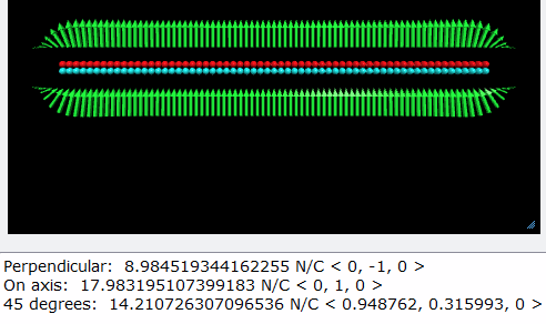
But given the above Python code, it might be fun to investigate a highly simplified capacitor approximated by a simple row of dipoles to see what happens in 2D. The code is here and the results are:

This is not an accurate reflection of how charges distribute themselves on a parallel plate capacitor, as there must be an increasing charge density when approaching the edges, and the above model doesn't accommodate this fact. Instead, it spreads them out completely evenly. Also, the plates are infinitely thin in this example and in reality they are not. (Finite thickness conducting plates must have charge on their outer faces because the line integral of the electrostatic field around any closed path must vanish.) But it is still interesting.
An exaggerated but also illustrative example would be more like this:

For more information on this topic, see "Electric field outside a parallel plate capacitor," by G. W. Parker, 2002, American Journal of Physics, 70(5), 502-507, doi:10.1119/1.1463738.
The point I'd also like to emphasize is the power of using VPython and Glowscript Trinket (tikz stuff) for physics modeling.
In fact, there's a book on the topic of Python generally for physics called, "Essential Python for the Physicist," by Giovanni Moruzzi, 2020.

