Gaussian Function Fourier Transform (Matlab)

Question

I am trying to write my own Matlab code to sample a Gaussian function and calculate its DFT, and make a plot of the temporal Gaussian waveform and its Fourier transform.

According to the FT pair:

\$ e^{-at^2} \iff \sqrt{\frac{\pi}{a}} e^{- \pi^2 \nu^2 /a}, \$

The FT of a Gaussian is a Gaussian, and it should also be a real function.

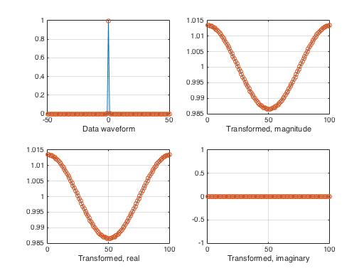
So here is my graph:

So, why is my FT a flat line instead of being Gaussian?

And why is it that when I plot the argument of the DFT, the imaginary part is nonzero? Shouldn't the FT be real?

Any help would be greatly appreciated.

Here is my code:

clear; clf; clc;
a=5;
n=50; % Length of DFT
k=[-n:1:n];

x=exp(-a.*k.^2); % Gaussian function

subplot(221);
plot(k,x);grid;
axis([1.5,n,-max(-x),max(x)]);
xlabel('Data waveform');
hold on; plot(k,x,'o'); hold off;

xx=fft(x)/n;
subplot(222);
plot(k, abs(xx));grid;xlabel('Transformed, magnitude');
axis([1,n,0,1]);
hold on; plot(k,abs(xx),'o'); hold off;

subplot(223);

plot(k, real(xx));grid;xlabel('Transformed, real');
hold on; plot(k, real(xx), 'o'); hold off;
axis([1,n,-1,1]);

subplot(224)
plot(k,imag(xx)); grid;
axis([1,n,-1,1]);
xlabel('Transformed, imaginary');
hold on; plot(k, imag(xx), 'o'); hold off;

figure(gcf);

Answer 1

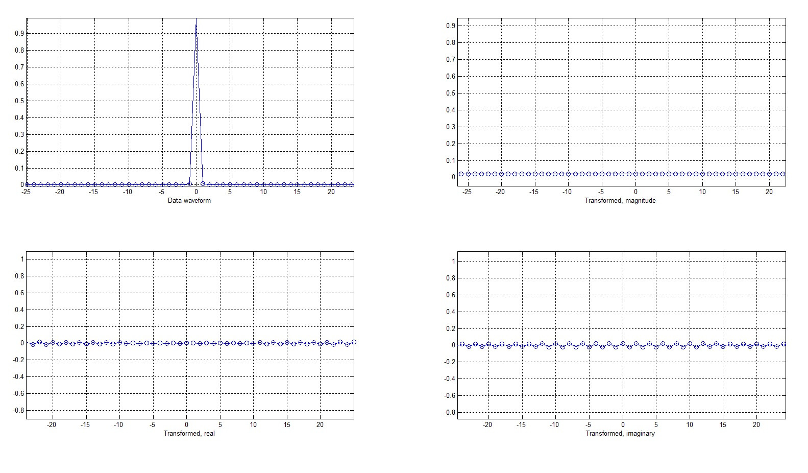
The FFT looks flat, because the value of your a is too high.

Secondly, you should use a different x-axis for the FFT plot. With N+1 time values, you get FFT points for nu values from -N/2 to +N/2.

You should know, that the vector, which the Matlab FFT function returns has these points in the order [0,1,2,...,+N/2,-N/2,...,-1]. This means you have to shift the vector in order to look like a Gaussian.

I would recommend, don't scale the axis manually for a first test.

There are imaginary parts, because of how the Gaussian is represented in the Matlab vector. More info here. You can use x = circshift(x,[0 -50]); to get a FFT without imaginary parts.

clear; clf; clc;
a=5;
n=50; % Length of DFT
k=[-n:1:n];

x=exp(-a.*k.^2); % Gaussian function
xs = circshift(x,[0 -50]); 

subplot(221);
plot(k,x);grid;
%axis([1.5,n,-max(-x),max(x)]);
xlabel('Data waveform');
hold on; plot(k,x,'o'); hold off;

nu=[0:1:2*n];
xx=fft(xs);
subplot(222);
plot(nu, abs(xx));grid;xlabel('Transformed, magnitude');
%axis([1,n,0,1]);
hold on; plot(nu,abs(xx),'o'); hold off;

subplot(223);

plot(nu, real(xx));grid;xlabel('Transformed, real');
hold on; plot(nu, real(xx), 'o'); hold off;
%axis([1,n,-1,1]);

subplot(224)
plot(nu,imag(xx)); grid;
%axis([1,n,-1,1]);
xlabel('Transformed, imaginary');
hold on; plot(nu, imag(xx), 'o'); hold off;

figure(gcf);