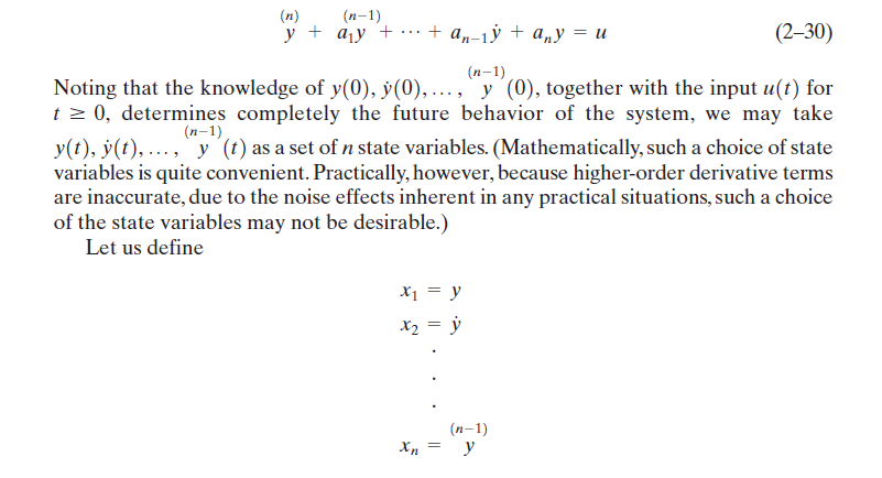
I'm confused about state-space state variables. How come knowing the initial conditions with the input 'determine completely the future behavior of the system'? From such knowledge, I can only approximate the 'next' state at 0+dt...
Also, how come knowing the designated n state variables at an arbitrary time t with the input suffice? It seems to me that there is an assumption that the highest order derivative vanishes?
For example, a one-dimensional moving ball system. At rest, this ball has a position x_0 and so only requires one state to be described fully. A constant speed moving ball needs one more state, namely the velocity. Now also if the velocity is changing, we need an additional state and so on. I understand this logic where knowing the highest order state allows us to climb down in knowing the lower order states one by one...For other systems, however, highest order derivates aren't necessarily constant, and so the even higher don't vanish.
I probably have some ideas gobbled and mixed up that need fixing.
Picture Source: Ogata's Modern Control Engineering
-
1\$\begingroup\$ If the state space model of a system is known, and is linear and time invariant, and if you also know the initial conditions, and the input signal, then of course you can determine the response at any time in the future. \$\endgroup\$– ChuCommented Sep 15, 2020 at 16:45
1 Answer
How come knowing the initial conditions with the input 'determine completely the future behaviour of the system'? From such knowledge, I can only approximate the 'next' state at 0+dt...
If you have \$u(t)\$ for future \$t\$, you can continue calculating the output at \$(0+dt+dt)\$, \$(0+dt+dt+dt)\$ etc. If I am not mistaken, being able to propagate the solution of a differential equation for future time is termed in text books as "existence and uniqueness of solutions to ODEs". It is guaranteed under suitable assumptions.
It seems to me that there is an assumption that the highest order derivative vanishes?
It doesn't. It's just that you don't need any higher derivatives since the \$n^{th}\$ derivative onwards can be represented in terms of the lower order ones (and input profile). What is that dependence, you ask ? It's given in the system description itself!
$$ y^{(n)} = u + \sum_{i=0}^{n-1}-a_i y^{(i)} $$
What about higher derivatives ?
$$ \begin{align} y^{(n+1)} ={} & \frac{d\ y^{(n)}}{dt} \\ ={} & \frac{d}{dt} \left(u + \sum_{i=0}^{n-1}-a_i y^{(i)}\right) \\ ={} & \frac{du}{dt} + \frac{d}{dt} \sum_{i=0}^{n-1}-a_i y^{(i)}\\ ={} & \frac{du}{dt} + \frac{d}{dt} \sum_{i=0}^{n-2}-a_i y^{(i)} -a_{n-1}\color{red}{y^{(n)}}\\ \end{align} $$
The last term (highlighted in red colour) can be replaced by the lower derivatives and finally you need only the lower derivatives (and the input profile) to represent any higher derivatives. They don't disappear, just get replaced with lower order equivalent.
For linear differential equations (and possibly even non linear), there is some underlying linear algebra concept where the higher order derivatives are linearly-dependent on the lower ones and you are effectively working in a space with only \$n\$ dimensions and you can't escape from it.
Example
Higher order derivatives don't vanish. They can be seen to be replaceable by lower order ones. A simple example is
$$\frac{d^2}{dt^2}y(t) + y(t) = 0$$
has solutions of the form
$$\begin{align} y(t) = & A\cos(t) + B\sin(t)\\ y^{(1)} = & -A\sin(t) + B\cos(t)\\ y^{(2)} = & -A\cos(t) - B\sin(t) & ={} & -y(t)\\ y^{(3)} = & A\sin(t) - B\cos(t) & ={} & -y^{(1)}(t)\\ y^{(4)} = & A\cos(t) + B\sin(t) & ={} & y(t)\\ y^{(5)} = & -A\sin(t) + B\cos(t) & ={} & y^{(1)}(t)\\ \end{align} $$ and so on.
For example, a one-dimensional moving ball system. At rest, this ball has a position x_0 and so only requires one state to be described fully. A constant speed moving ball needs one more state, namely the velocity. Now also if the velocity is changing, we need an additional state and so on.
You are partially right. This is only correct if you don't have any laws governing the moving body. In the absence of any laws governing the moving body, to represent a curve \$x(t)\$, you need all higher derivatives of the curve (i.e. the Taylor series expansion of the curve \$x(t_0+\Delta t) = \sum_{i=0}^{\infty}c_i \Delta t \cdot x^{(i)}(t_0)\$). But, if you have a law governing the curve such as newton's law
$$\frac{d^2 x(t)}{dt^2} = u(t) = \frac{f(t)}{m}$$
With this law in hand, all higher derivatives can be represented in terms of lower derivatives (and the input profile) as mentioned earlier in this answer.

