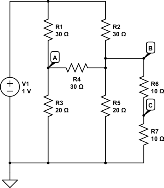
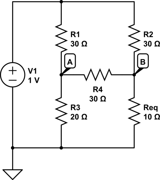
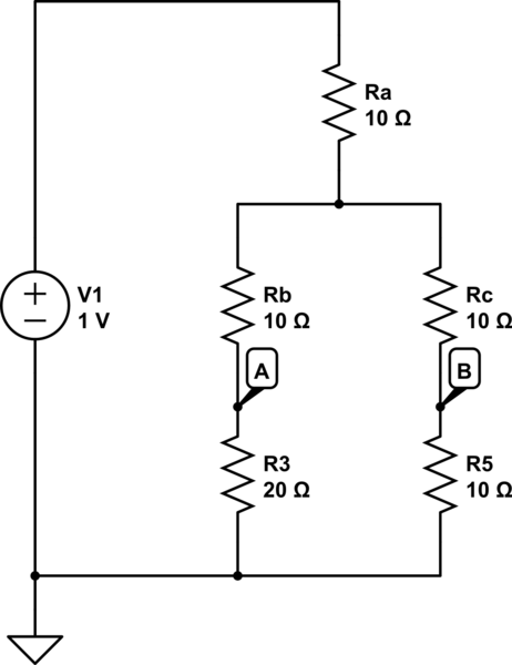
Some may say, there is no common approach but there must at least be
algorithm since computers can do the job all the time.
More than a few ways. But time for just one. Since you bring up that computers do this routinely, then:
Graph Theory: Spice-Like
We'll follow a concrete example from start to finish to help illustrate a method that is similar to what Spice programs use. It's not the exact same method. But your resistor case is a subset of the problems Spice handles and for these cases the method I'll discuss is quite close enough that the differences are negligible.
If you want more specific details about how Spice programs approach this in more general cases, then please see "SPICE2: A Computer Program to Simulate Semiconductor Circuits" by Laurence W. Nagel, directly from Berkeley. This one is entirely free. Just click on the PDF link at that site. The details are addressed quite early in the text. So feel free.
Concrete Example
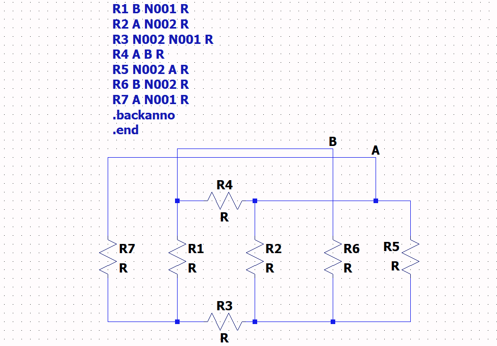
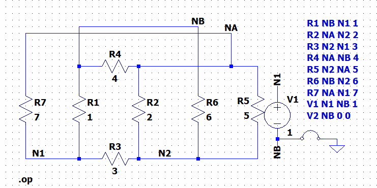
Here's a schematic in LTspice, including its netlist:

This netlist is in simple ASCII text. You can parse it, trivially. And I mean trivially! There are 7 lines you care about, obviously. Just write up a routine to read any resistor netlist saved by LTspice (or any Spice program, as all of them support these netlist Spice cards.) Make sure to label the two nodes that you care about making your measurement from. I've called them A and B but obviously you can make up anything you want, there.
Its Directed Graph: aka Incidence Matrix
The code you write (or the method you would use by hand) just converts the above to this directed graph matrix:
$$
\begin{matrix}
\quad\fbox{A} & \\
& \begin{matrix}
& & \text{nodes} \\
& & \overbrace{\begin{matrix}N_1 & N_2 & N_A & N_B\end{matrix}}
\\
\text{edges}&\left\{\begin{matrix}R_1\\R_2\\R_3\\R_4\\R_5\\R_6\\R_7\end{matrix}\right.&
\left[\quad\begin{matrix}
\vphantom{R_1}\hfill 1 & \hfill 0 & \hfill 0 & \hfill -1 \\
\vphantom{R_1}\hfill 0 & \hfill 1 & \hfill -1 & \hfill 0 \\
\vphantom{R_1}\hfill 1 & \hfill -1 & \hfill 0 & \hfill 0 \\
\vphantom{R_1}\hfill 0 & \hfill 0 & \hfill -1 & \hfill 1 \\
\vphantom{R_1}\hfill 0 & \hfill -1 & \hfill 1 & \hfill 0 \\
\vphantom{R_1}\hfill 0 & \hfill 1 & \hfill 0 & \hfill -1 \\
\vphantom{R_1}\hfill 1 & \hfill 0 & \hfill -1 & \hfill 0
\end{matrix}\quad\right]
\end{matrix}
\end{matrix}
$$
All I did was to read a line (by eye, obviously) and place a -1 for the first node and a +1 for the second node shown in the netlist for each part. Everything else gets 0. This is just falling off a log. Anyone can do this. And so can a very short piece of code.
Using freely available SymPy and SageMath for this, running on a variety of environments and using the Python language, write:
A = Matrix([[1,0,0,-1],[0,1,-1,0],[1,-1,0,0],[0,0,-1,1],
            [0,-1,1,0],[0,1,0,-1],[1,0,-1,0]])
You could, of course, generate that code automatically. And you may generate it as initializers for a matrix in any other language of your own choosing. Could not be easier.
Its Conductance Matrix
You will need a diagonal conductance matrix. This one is still easier (as if that were possible):
$$
\begin{matrix}
\quad\fbox{C} & \\
& \begin{matrix}
& \begin{matrix}R_1 & R_2 & R_3 & R_4 & R_5 & R_6 & R_7\end{matrix}
\\
\begin{matrix}R_1\vphantom{\frac1{R_1}}\\R_2\vphantom{\frac1{R_1}}\\R_3\vphantom{\frac1{R_1}}\\R_4\vphantom{\frac1{R_1}}\\R_5\vphantom{\frac1{R_1}}\\R_6\vphantom{\frac1{R_1}}\\R_7\vphantom{\frac1{R_1}}\end{matrix}&
\left[\quad\begin{matrix}
\frac1{R_1} \\
& \frac1{R_2} & & & & \large{0} \\
& & \frac1{R_3} \\
& & & \frac1{R_4} \\
& & & & \frac1{R_5} \\
& \large{0} & & & & \frac1{R_6} \\
& & & & & & \frac1{R_7}
\end{matrix}\quad\right]
\end{matrix}
\end{matrix}
$$
Coded up as:
var('r1 r2 r3 r4 r5 r6 r7')
C = Matrix([[1/r1,0,0,0,0,0,0],[0,1/r2,0,0,0,0,0],[0,0,1/r3,0,0,0,0],
            [0,0,0,1/r4,0,0,0],[0,0,0,0,1/r5,0,0],[0,0,0,0,0,1/r6,0],
            [0,0,0,0,0,0,1/r7]])
The above conductance matrix can also include capacitors and inductors, as well. But the details applied by Spice programs become more nuanced and it's better that you refer to "SPICE2: A Computer Program to Simulate Semiconductor Circuits" by Laurence W. Nagel for some expansion.
For now, let's just move on with simple conductance matrices built only from resistor values.
General Matrix Solution Equation and the Schur Complement
It turns out that the product, \$A^T\,C\,A\$, always results in a square symmetric matrix seen as this block matrix:
$$W=A^T\,C\,A=\left[\begin{matrix}P&Q^T\\Q&R\end{matrix}\right]$$
At this point, we've two choices. Either choice works just fine. One is that we set \$v_a=1\:\text{V}\$ and \$v_b=0\:\text{V}\$ and find out what currents we get. The other is that we set the KCL sum at \$v_a\$ to be \$1\:\text{A}\$ and at \$v_b\$ to be \$-1\:\text{A}\$ and find out what the resulting node voltages are for \$v_a\$ and \$v_b\$.
If we set the currents and solve for all the node voltages, the matrix solution is harder since you need to invert a larger matrix. So it's better (my view) to set the node voltages and find out what the resulting currents will be. This allows the use of the Schur complement.
So we will instead just set \$v_a=1\:\text{V}\$ and \$v_b=0\:\text{v}\$ and solve for the complementary currents (what enters must be the same as what leaves.) The value, \$R_{total}=\frac{1\:\text{V}}{I}\$, will be the resistance.
The full-blown setup follows (made with MiKTeX and Latex code I learned about here):

(Note that you would likely use numerical values for \$C\$ and so \$W\$ wouldn't look that complicated. It would just be some numbers there.)
We want to solve for \$\hat{i}\$. We don't care about \$\hat{v}\$, as it really doesn't matter to us. So we use the Schur complement to avoid having to solve for \$\hat{v}\$ (since we don't care about it.) By ignoring what we don't care about, the computation problem is made simpler.
The Schur complement is trivial to derive. Note that (1) \$P\hat{v}+Q^T\hat{e}=\hat{0}\$ and (2) \$Q\hat{v}+R\hat{e}=\hat{i}\$? From (1), solve as \$\hat{v}=-P^{-1}Q^T\hat{e}\$ and then substitute that into (2):
$$\begin{align*}
\hat{i}&=Q\hat{v}+R\hat{e}
\\\\
&=Q\left(-P^{-1}Q^T\hat{e}\right)+R\hat{e}
\\\\
&=-QP^{-1}Q^T\hat{e}+R\hat{e}
\\\\
&=R\hat{e}-QP^{-1}Q^T\hat{e}
\\\\
&=\left(R-QP^{-1}Q^T\right)\hat{e}
\end{align*}$$
And that's the Schur complement.
Do note that it reduces the size of the required matrix inversion, this way. Just a 2x2 rather than inverting an entire 4x4 (which would succeed at getting the right results, but is generally more work because it also solves for those two voltages, \$v_1\$ and \$v_2\$, which we really don't need to know.)
Also, you can easily invert a 2x2 by hand. Not so much with a 4x4, where it starts to get more painful.
Performing the Indicated Computations
So here's the remaining code. I'll later then assign values to each of the resistors where their value is the same as their identification number and get some results.
W = A.T * C * A                    # square symmetric block matrix
P = W.extract([0,1],[0,1])         # P-block
Q = W.extract([2,3],[0,1])         # Q-block
R = W.extract([2,3],[2,3])         # R-block
excite = Matrix([1,0])             # excitation of 1 V and 0 V
for u in list(( R - Q * P.inv() * Q.T) * excite ):
    u.subs({ r1:1, r2:2, r3:3, r4:4, r5:5, r6:6, r7:7 })
315/523
-315/523
So, we'd find that the total resistance is \$\frac{1\:\text{V}}{I=\frac{315}{523}\:\text{A}}=\frac{523}{315}\:\Omega\approx 1.66\:\Omega\$.
That's it. Seriously.
(Note for later that \$I=\frac{315}{523}\:\text{A} \approx 602.294\:\text{mA}\$.)
Trust, but Verify!
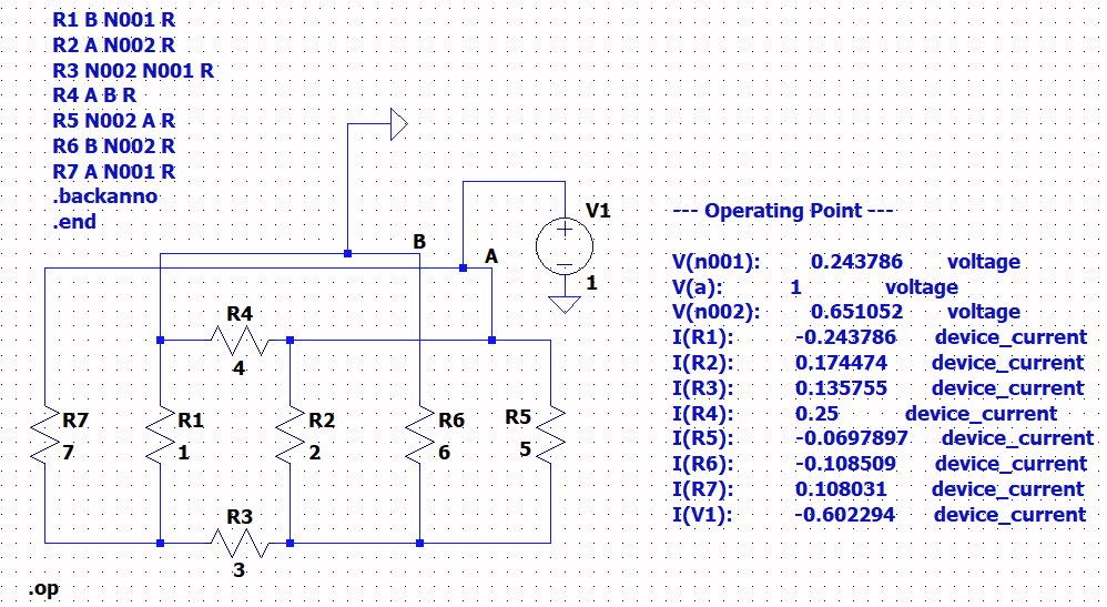
So, let's verify. Here's the initial schematic modified to include all the extra stuff needed to get a numerical solution:

Note that the current leaving the voltage supply has the magnitude of \$602.294\:\text{mA}\$ and that \$\frac{1\:\text{V}}{602.294\:\text{mA}}\approx 1.66\:\Omega\$.
And that is a match!!!
(And the current is also seen to have matched, too.)
Summarizing the Algorithm
So, here's what you need to do:
- Define for yourself a line by line way of listing out the resistors and the nodes they connect up with. This is called a netlist. You can use the Spice format for this -- it is what I'd choose to do because then I could just use the schematic editor to create any kind of crazy schematic. And it would support other methods of generating netlists beyond the use of the Spice schematic editor. You don't have to do that. You can create your own format. Doesn't matter. You just need something simple to work with.
- Write code to read what you produce for step #1 and generate a directed graph matrix \$A\$ from it.
- Write extremely simple code to produce the conductance matrix \$C\$.
- Using the matrix math I've pointed out above, solve for the resulting current that is developed.
- Divide that current into the \$1\:\text{V}\$ excitation supplied to the network to get the resistance.
That's all there is.
There are other ways. But this one is straight forward and will handle any set of cases you present, so long as it is a fully connected graph.
Fully Connected Graphs: What???
Well, there are methods you can apply to the incidence matrix, \$A\$, to verify this.
For example, looking at its right nullspace will tell you if it is fully connected:
pprint(A.nullspace())
⎡⎡1⎤⎤
⎢⎢ ⎥⎥
⎢⎢1⎥⎥
⎢⎢ ⎥⎥
⎢⎢1⎥⎥
⎢⎢ ⎥⎥
⎣⎣1⎦⎦
Getting only one vector with all 1's tells you this is a fully connected graph. This vector says that the only way to get zero currents (the KCL null-space) is to have all of the existing nodes set to the same voltage. All of them. Not just some of them. (Otherwise, you'd see more vectors here.)
(Oh, I should include a short synopsis. So here is a description of the four fundamental subspaces for a short summary.)
Added Value for Graph Theory: Meshes!
It's easy to find the independent meshes using the left null-space:
pprint(A.T.nullspace())
⎡⎡1 ⎤  ⎡0⎤  ⎡-1⎤  ⎡0 ⎤⎤
⎢⎢  ⎥  ⎢ ⎥  ⎢  ⎥  ⎢  ⎥⎥
⎢⎢-1⎥  ⎢1⎥  ⎢0 ⎥  ⎢-1⎥⎥
⎢⎢  ⎥  ⎢ ⎥  ⎢  ⎥  ⎢  ⎥⎥
⎢⎢-1⎥  ⎢0⎥  ⎢1 ⎥  ⎢-1⎥⎥
⎢⎢  ⎥  ⎢ ⎥  ⎢  ⎥  ⎢  ⎥⎥
⎢⎢1 ⎥, ⎢0⎥, ⎢0 ⎥, ⎢0 ⎥⎥
⎢⎢  ⎥  ⎢ ⎥  ⎢  ⎥  ⎢  ⎥⎥
⎢⎢0 ⎥  ⎢1⎥  ⎢0 ⎥  ⎢0 ⎥⎥
⎢⎢  ⎥  ⎢ ⎥  ⎢  ⎥  ⎢  ⎥⎥
⎢⎢0 ⎥  ⎢0⎥  ⎢1 ⎥  ⎢0 ⎥⎥
⎢⎢  ⎥  ⎢ ⎥  ⎢  ⎥  ⎢  ⎥⎥
⎣⎣0 ⎦  ⎣0⎦  ⎣0 ⎦  ⎣1 ⎦⎦
Shows you one set of independent meshes in the circuit's directed graph. There are four, in this case. These can be combined in various ways to find other meshes. But there will only be four independent ones, regardless.
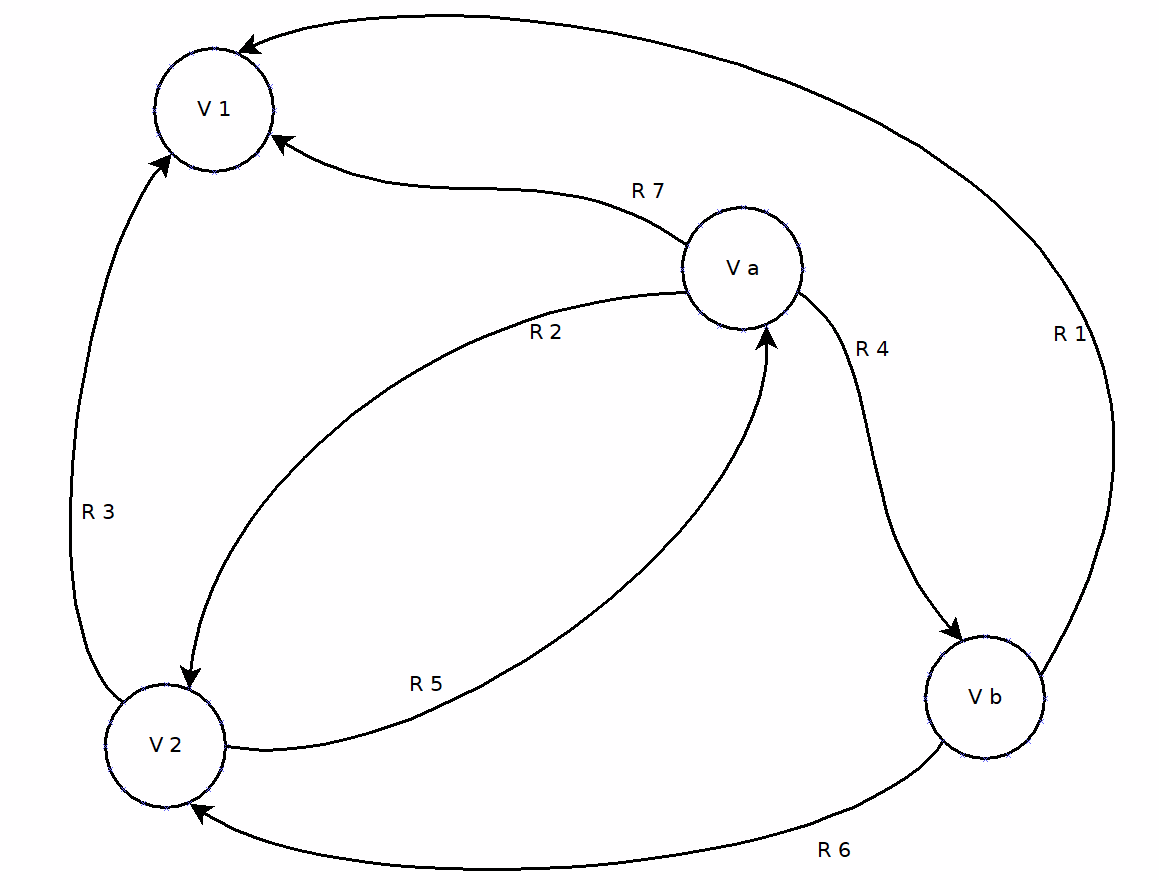
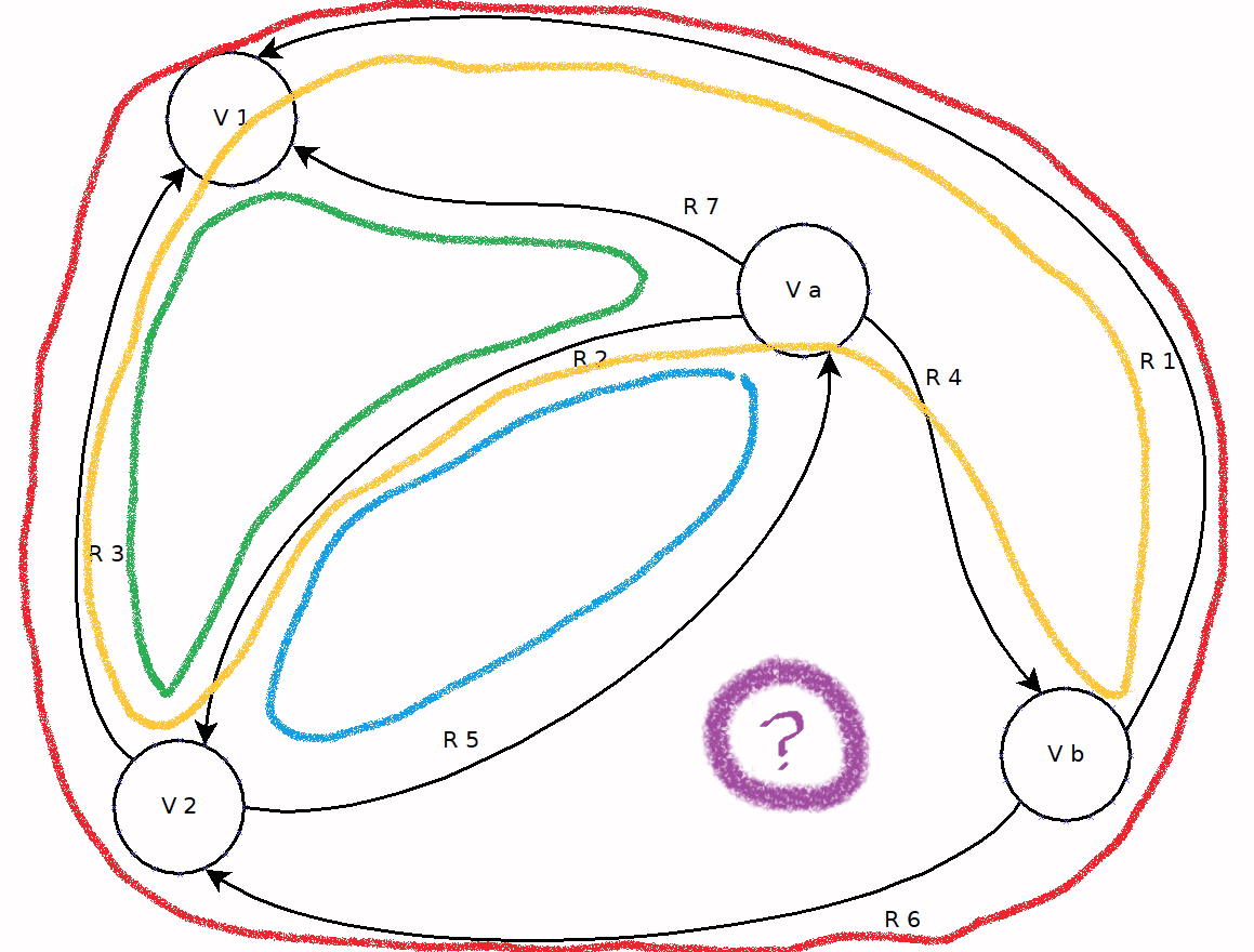
Looking at the circuit's directed graph (made with freely available Dia):

The first column vector above tells you that if you follow edge \$R_1\$ with its arrow, then go oppositely against \$R_3\$, then go oppositely against \$R_2\$, and then go with \$R_4\$, that you will have one mesh there. The second column vector says with \$R_2\$ and with \$R_5\$ is another mesh. (Parallel resistor pair.) The third column vector says against \$R_1\$, with \$R_6\$, with \$R_3\$ is another mesh. And the fourth column vector says against \$R_2\$, with \$R_7\$, against \$R_3\$ is another mesh.
These four meshes are colored in below:

Oh! Wait.
I added a 5th one, didn't I? The purple circle.
What about that mesh?
Well, it's just the sum of the yellow (1st), blue (2nd), and red (3rd) meshes. Let's double-check that:
U = A.T.nullspace()
pprint( U[0] + U[1] + U[2] )
⎡0⎤
⎢ ⎥
⎢0⎥
⎢ ⎥
⎢0⎥
⎢ ⎥
⎢1⎥
⎢ ⎥
⎢1⎥
⎢ ⎥
⎢1⎥
⎢ ⎥
⎣0⎦
Yup! Perfect.
So it seems that other meshes can be constructed from these independent ones.
If we added this one to the list and deleted the red one, then we'd still have four independent meshes that span the same KVL nullspace.
So you can add or subtract meshes to make other meshes.
But it takes exactly four independent ones, in this case, to span the KVL (left) null-space. If more than four, then at least one mesh must be dependent on others in the list.
This is because the rank of this incidence matrix \$A\$ is 3. Given that there are 7 rows, this means \$7-3=4\$ vectors required to span its KVL null-space. So long as the vectors are the minimum sufficient to span that null-space, you are good.
This is a cool way to find meshes needed to solve, when using the mesh method of analysis, by the way!
Final Note: Selecting Random Nodes
only given that the a voltage is applied between two random nodes.
The incidence matrix \$A\$ would keep all the rows just the same as before, since the rows correspond to resistors that are connected up into the circuit and you wouldn't be altering their topology.
So that stays the same.
But you would need to move the columns around so that the two nodes having the excitation applied to them are in the last two columns in order to avoid the need for horrible syntax.
(Technically, we could write some insane syntax. But let's avoid going there as it moves away from understanding things and towards language syntax geekland.)
For example, suppose we wanted to supply the excitation to the first and last nodes (\$v_1\$ and \$v_b\$) as shown in the following schematic:

The schematic topology is unchanged. So the rows in \$A\$ don't change, either. But the excitation can now be applied to any two nodes at will with the above schematic. In the case shown above, it's the first and last nodes of \$A\$.
The following code would take what has already been done above and apply it slightly differently (moving columns around with SymPy syntax) to get the desired result:
A1 = A[:,[1,2,0,3]]
W1 = A1.T * C * A1
P1 = W1.extract([0,1],[0,1])
Q1 = W1.extract([2,3],[0,1])
R1 = W1.extract([2,3],[2,3])
for u in list(( R1 - Q1 * P1.inv() * Q1.T) * excite ):
    u.subs({ r1:1, r2:2, r3:3, r4:4, r5:5, r6:6, r7:7 })
28/23
-28/23
(The [1,2,0,3] bit above says to build a new \$A\$ from the old \$A\$'s 2nd col, 3rd col, 1st col, and 4th col, in that order.)
So we find \$I=\frac{28}{23}\:\text{A}\approx 1.21739\:\text{A}\$.
A run of the above schematic shows:
I(V1): -1.21739 device_current
Which is the expected result.
(So the resistance in this case would be \$R_{total}\approx 821.43\:\text{m}\Omega\$. And given the value of \$R_1\$, we'd expect something less than 1 here.)
This exposition not only shows you how to develop a solution for one case, but also how to adjust it to ask about pairing any two selected nodes. The topology of the resistor circuit is unchanged. It's just some syntax changes needed to construct the right Schur complement matrices for the solution. That's all.
I'll provide a final demonstration that is more about the power of software like Python/Sympy than the power of graph theory. The power of graph theory is already shown. But this just puts a cap on the example resistor circuit I started with. So may as well.
I can define a function that accepts a list of the four nodes, but ordered in such a way that we test every node pair for its effective resistance:
def findR(L1):
    global A, C                      # access to our A and C matrices
    A1 = A[:, L1]                    # temp re-arranged A
    W1 = A1.T * C * A1               # temp symmetric block matrix
    P1 = W1.extract( [0,1], [0,1] )  # temp P-block
    Q1 = W1.extract( [2,3], [0,1] )  # temp Q-block
    R1 = W1.extract( [2,3], [2,3] )  # temp R-block
    return 1.0/list( ( R1 - Q1 * P1.inv() * Q1.T ) * Matrix([1,0])
                   )[0].subs({ r1:1, r2:2, r3:3, r4:4, r5:5, r6:6, r7:7 })
With that in hand I can now perform the following:
for u in [ list(set([0,1,2,3])-set(i))+list(i)
    for i in itertools.combinations([0,1,2,3],2)]:
        u, findR(u).n()
([2, 3, 0, 1], 1.48571428571429)
([1, 3, 0, 2], 1.67222222222222)
([1, 2, 0, 3], 0.821428571428571)
([0, 3, 1, 2], 1.09126984126984)
([0, 2, 1, 3], 1.59285714285714)
([0, 1, 2, 3], 1.66031746031746)
And there you have all of the allowable equivalent resistances for that circuit, using any pair of nodes. (The last two nodes listed are the ones being probed.)
Summary of Graph Theory
There's a lot you can do when you better understand how KCL, KVL, the column-space, row-space, and two null-spaces all play well together to describe circuits.
I hope this should be sufficient to motivate you to experiment on your own, firming this up in mind.
Further reading:
Wai-Kai Chen's "Graph Theory and Its Engineering Applications". The author assumes some maturity. But by the 2nd chapter you are off and running with circuit graphs that are practical and meaningful.
Gilbert Strang (anything by him is good and usually targeted at undergrads just learning this stuff), 5th edition, "Differential Equations and Linear Algebra". Gilbert Strang really can help you with understanding linear matrices, vector spaces, and their application to solutions. (He taught his last class, May of 2023, at the age of 88! A great many owe him so much for his dedication to those starting out on this kind of learning path. I owe him what I can never hope to pay back. My best to him!)
I've been sniped!

