How to sketch the Bode diagram of the output filter of a Buck converter?

Question

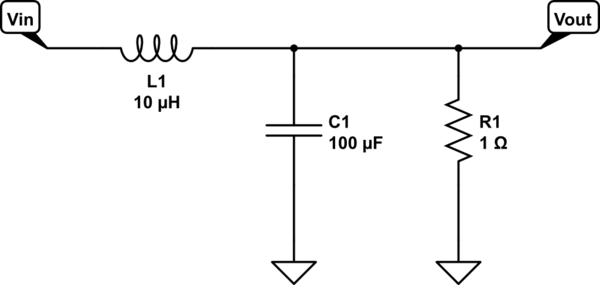
I'm trying to figure out the Bode diagram of the output filter of a Buck converter:

^{simulate this circuit – Schematic created using CircuitLab}

Vout is proportional to the current traversing the parallel impedance of the capacitor and resistor, Zrc, and the current is proportional to Vin and inversely proportional to the impedance of the inductance in series with the parallel of capacitor and resistor:

$$V_{out} = I \cdot Z_{RC} = \frac{V_{in}}{Z_L + Z_{RC}} \cdot Z_{RC}$$ $$Z_{rc} = \frac{1}{\frac{1}{Z_R} + \frac{1}{Z_R}}$$ $$V_{out} = \frac{V_{in}}{Z_L \cdot \left( \frac{1}{Z_C} + \frac{1}{Z_R} \right) + 1}$$

Replacing the impedance by their Laplace equivalents: $$\frac{V_{out}}{V_{in}} = \frac{R}{s^2RLC + sL + R}$$

Which looks quite familiar (and confirmed by this application note, page 10)

Now, how do I continue to sketch the Bode diagram? I know I should identify the poles, but with my values, the poles are in the i plane:

• L = 10µH
• C = 100µF
• R = 1Ω

Can someone give me a hint?

Answer 1

Background

Starting with your result and proceeding:

$$\begin{align*} H\left(s\right)&=\frac{R}{R\,L\,C\,s^2+L\,s+R}\\\\ &=\frac{1}{L\,C\,s^2+\frac LR\,s+1}\\\\ &=\frac{\frac 1 {L\,C}}{s^2+\frac 1{R\,C}s +\frac 1{L\,C}}\tag{1} \end{align*}$$

The denominator you see in equation (1) is sometimes called the characteristic equation. There are two relatively obvious time constants present there, \$\tau_{_0}=\sqrt{L\,C}\$ and \$\tau_{_1}={R\,C}\$, and therefore also two obvious angular frequencies, \$\omega_{_0}=\frac 1{\sqrt{L\,C}}\$ and \$\omega_{_1}=\frac 1{R\,C}\$.

So this would suggest the following:

$$\begin{align*} H\left(s\right) &=\frac{\omega_{_0}^2}{s^2+\omega_{_1}\,s +\omega_{_0}^2}\tag{2} \end{align*}$$

Standardized Form

Equation (2) isn't in standardized form, yet. And there's a good reason to do some more work. Equation (2) has two different angular frequencies and it's not clear how they might interact. Perhaps there's another way to express it that will help clarify things. Some kind of "standard form" that will be more readily meaningful?

The most interesting behaviors for equation (2) will be nearer where the denominator is zero and this is where focused attention would make sense. So let's solve the quadratic equation, \$\frac{-b\pm\sqrt{b^2-4\:a\:c}}{2\:a}\$. A quick glance suggests setting \$\alpha=\frac 12\omega_{_1}\$. Then we have \$s_1=-\alpha+\sqrt{\alpha^2-\omega_{_0}^2}\$ and \$s_2=-\alpha-\sqrt{\alpha^2-\omega_{_0}^2}\$ or else, written another way, \$s_1=-\alpha+j\sqrt{\omega_{_0}^2-\alpha^2}\$ and \$s_2=-\alpha-j\sqrt{\omega_{_0}^2-\alpha^2}\$. If we now set the damped angular frequency as \$\omega_d=\sqrt{\omega_{_0}^2-\alpha^2}\$ then \$s_1=-\alpha+j\,\omega_d\$ and \$s_2=-\alpha-j\,\omega_d\$.

If \$\alpha=\omega_{_0}\$ then \$\omega_d=0\$ and the system is critically-damped, with \$s_1=s_2=-\alpha\$, and both obviously the same real value. If \$\alpha\gt\omega_{_0}\$ then \$\omega_d\$ is imaginary and the system is over-damped, with \$s_1\ne s_2\$ but both real-valued. If \$\alpha\lt\omega_{_0}\$ then \$\omega_d\$ is real and the system is under-damped, \$s_1\$ and \$s_2\$ being complex conjugates.

Before proceeding further, it's worth looking again at \$\omega_d=\sqrt{\omega_{_0}^2-\alpha^2}\$. This can be expressed instead as \$\omega_d=\omega_{_0}\sqrt{1-\left[\frac{\alpha}{\omega_{_0}}\right]^2}\$. If we now set \$\zeta=\frac{\alpha}{\omega_{_0}}\$ (a dimensionless value) then \$\omega_d=\omega_{_0}\sqrt{1-\zeta^2}\$. It also then follows that \$\alpha=\zeta\,\omega_{_0}\$.

To zero in on the poles, the interesting areas surrounding the location where the denominator is zero, let's reformulate equation (2) above:

$$\begin{align*} H\left(s\right) &=\frac{\omega_{_0}^2}{\left(s-s_1\right)\cdot\left(s-s_2\right)}\\\\ &=\frac{\omega_{_0}^2}{\left(s-\left[-\alpha+j\,\omega_d\right]\right)\cdot\left(s-\left[-\alpha-j\,\omega_d\right]\right)}\\\\ &=\frac{\omega_{_0}^2}{s^2+2\,\alpha\,s+\alpha^2+\omega_d^2}=\frac{\omega_{_0}^2}{\left(s+\alpha\right)^2+\omega_d^2}\\\\ &=\frac{\omega_{_0}^2}{s^2+2\,\zeta\,\omega_{_0}\,s+\left(\zeta\,\omega_{_0}\right)^2+\omega_{_0}^2\left(1-\zeta^2\right)}\\\\ &=\frac{\omega_{_0}^2}{s^2+2\,\zeta\,\omega_{_0}\,s+\omega_{_0}^2}\tag{3} \end{align*}$$

This is the standardized form (except it is missing the gain, \$K\$) and something significant has been achieved here. We now have a single angular frequency, \$\omega_{_0}\$, and a new dimensionless damping factor, \$\zeta\$. If \$\zeta=1\$ then the system is critically damped. If \$\zeta \gt 1\$ then the system is over-damped. If \$\zeta\lt 1\$ then the system is under-damped.

Note 1: There is something else called a damping value (or in Sallen and Key's writings it is called a dissipation factor), which has units. It is designated by the letter \$d\$ and not \$\zeta\$. So be cautious when reading. Earlier writing will often use the damping value or dissipation factor, \$d\$. This will be particularly true for earlier authors who are familiar with Sallen and Key's, "A Practical Method of Designing RC Active Filters", Technical Report No. 50 (now unclassified.) Newer books have evolved to use the above approach and therefore have now tended to standardize on using the unitless damping factor, \$\zeta\$, together with \$\omega_{_0}\$, instead.

---

Note 2: If you want to study the filter behavior without getting bogged down by the angular frequency itself, just set \$\omega_{_0}=1\:\frac{\text{rad}}{\text{s}}\$. The equation is a lot simpler now, \$H\left(s\right)=\frac{1}{s^2+2\,\zeta\,s+1}\$ and there's only one parameter to play with, \$\zeta\$. The amplitude is then:

\$\frac{e_\text{out}}{e_\text{in}}=-20\operatorname{log}_{10}\left(\sqrt{\omega^4+\left(4\,\zeta^2-2\right)\omega^2+1}\right)\$

If you plug in \$\omega=1\:\frac{\text{rad}}{\text{s}}\$ you'll find that the under-damped peak value is \$\frac{e_\text{out}}{e_\text{in}}=-20\operatorname{log}_{10}\left(2\,\zeta\right)\$. The phase response is also now just \$\phi=\operatorname{tan}^{-1}\left(\frac{2\,\zeta\,\omega}{1-\omega^2}\right)\$. So these two things make it very easy to study the amplitude and phase response in this special case. But once you know the case where \$\omega_{_0}=1\:\frac{\text{rad}}{\text{s}}\$, you have already studied every possible other value for \$\omega_{_0}\$. All you have to do is "re-normalize" things to different values of \$\omega_{_0}\$. What you learned from \$\omega_{_0}=1\:\frac{\text{rad}}{\text{s}}\$ covers every other case. So just keep it simple while studying.

Your Question

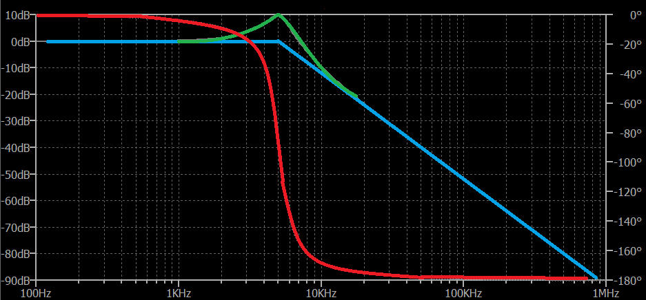
In your case, the unitless damping factor is \$\zeta=\frac \alpha{\omega_0}\approx 0.158\$ and this means it's under-damped. From this, you can work out the peaking to be \$-20\operatorname{log}_{10}\left(2\zeta\right)\approx +10\:\text{dB}\$. You also know this is of \$2^\text{nd}\$ order, so the behavior at angular frequencies far higher than \$\omega_{_0}\approx 31.623\:\text{k}\frac{\text{rad}}{\text{s}}\$ drops off at \$-40\:\frac{\text{dB}}{\text{decade}}\$. At angular frequencies far less than \$\omega_{_0}\$, the magnitude will be \$0\:\text{dB}\$. And in general, far less means \$\lt \frac1{10}\,\omega_{_0}\$ and far more means \$\gt 10\,\omega_{_0}\$. Right at \$\omega_{_0}\$, the peak will be at \$+10\:\text{dB}\$ (as already mentioned.)

Given this is \$2^\text{nd}\$ order, you'll expect to see the phase flat and close to \$0^\circ\$ at \$\frac1{10}\,\omega_{_0}\$, curving rapidly towards \$-90^\circ\$ at approximately \$\omega_{_0}\$ (where the inflection point is at), and then curving back towards flat again at \$-180^\circ\$ at \$10\,\omega_{_0}\$.

I've hand-drawn a starting blue line to show the basic case without peaking. Just straight lines to the corner frequency (about \$5\:\text{kHz}\$.) The green bit is a hand-drawn bit of peaking to the computed peak value. The red line started out as three separate straight lines: one on the left to about \$500\:\text{Hz}\$ at \$0^\circ\$, another on the right going from about \$50\:\text{kHz}\$ and higher, and a third showing a rapid dive (almost but not quite vertical) going through \$-90^\circ\$ at \$5\:\text{kHz}\$. The rest was sketched in to connect those up. All such \$2^\text{nd}\$ order plots look the same. It's just positioning with values that makes one different from another. (The sharpness of the phase change is greater with higher peaking. Lower peaking will have a more gradual phase change. I'll leave the details for you to work out over time.)

None of this addresses your buck converter as a system. But it covers your output filter.

Answer 2

When it comes down to analyzing the transfer function of a buck converter operated in voltage-mode control, you have to include parasitics around the inductor and the capacitor: \$r_L\$ for the inductor and \$r_C\$ for the capacitor. The circuit can be further refined by adding the transistor \$r_{DS(on)}\$ and the diode dynamic resistance \$r_d\$ respectively weighted by \$D\$ and \$(1-D)\$ but it complicates the circuit a little more. Actually, to model the quality factor \$Q\$ adequately, one should also account for switching losses on the transistor and diode (\$t_{rr}\$) plus magnetic losses: all these losses participate in lowering the resonating peak as these elements dissipate energy in heat and damp the system. Nobody does that as it would be extraordinary complicated to derive and, in the end, you have to measure the circuit transfer function with a real prototype naturally accounting for all these contributors.

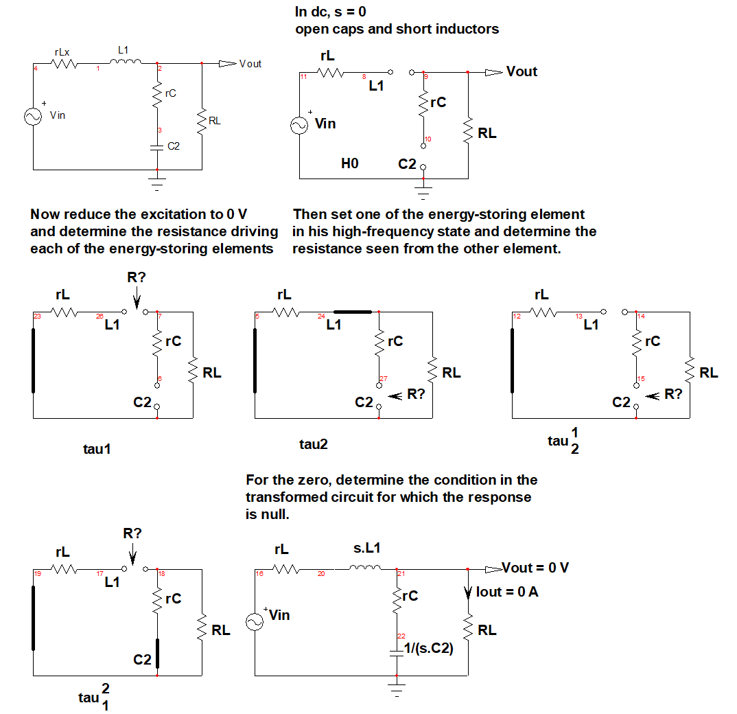
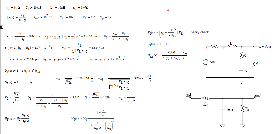
Regarding the determination of the upgraded \$LC\$ filter, look at the below figure which explains how the fast analytical circuits techniques or FACTs can help you determine it without writing a line of algebra. As documented in the book I wrote on FACTs, the transfer function must comply with the low-entropy format defined as follows: \$H(s)=H_0\frac{1+\frac{s}{\omega_z}}{1+\frac{s}{Q\omega_0}+(\frac{s}{\omega_0})^2}\$. In this format, the leading term \$H_0\$ must have the same unit as the transfer function you want to determine. For a voltage gain expressed in [V]/[V], it is unitless but would be \$\Omega\$ for an impedance, \$S\$ for an admittance etc.

You start observing the circuit for \$s=0\$ where the capacitor is open and the inductor is replaced by a short circuit. The transfer function in this mode is \$H_0\$ and involves a simple resistive divider (in which you see that \$r_L\$ plays a role). Then, reduce the excitation to 0 V (replace the source by a short circuit) and "look" at the resistance offered by each energy-storing elements terminals when temporarily removed from the circuit. This gives you the low-frequency time constants. Then, set one of the time constant in its high-frequency state (a short circuit for a cap. or an open circuit for an inductor) and determine the resistance "seen" through the connections of the remaining element. This is it, if you assemble the time constants as shown in the below Mathcad file, you have the denominator.

Regarding the zero, it is contributed by the combination \$r_C\$ and \$C_2\$. They form an impedance \$Z=r_C+\frac{1}{sC_2}\$. When this impedance equals 0 \$\Omega\$ for \$s=s_z\$ then this is your zero. In this mode, the stimulus does not give rise to a response and is lost somewhere in the circuit: \$r_C\$ and \$C_2\$ from a transformed short circuit when \$s=s_z\$. And you see why the presence of \$r_C\$ is important as it produces a zero which softens the frequency response and provides phase boost at crossover. You can now plot the frequency response and explore a point where to crossover:

With a 5-kHz resonant frequency, you need to close the loop so that enough gain exists at the resonance and damps the \$LC\$ filter. A crossover of 15 kHz would be adequate as a start for this converter. As you can see, the FACTs can determine the transfer function in a swift and efficient manner without writing a single line of algebra. Furthermore, they lead to a low-entropy expression naturally highlighting the presence of poles, zeroes and gain if any.