0
\$\begingroup\$

I am trying to replicate a result from a textbook that I am using to study input filter design for buck converters. enter image description here
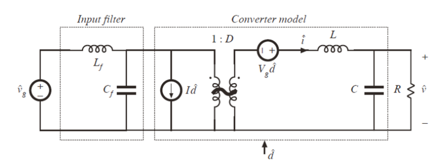
The parameters for the converter and filter are as follows:

  • D = 0.5
  • L = 100 μH
  • C = 100 μF
  • R = 3 Ω
  • Lf = 330 μH
  • Cf = 470 μF

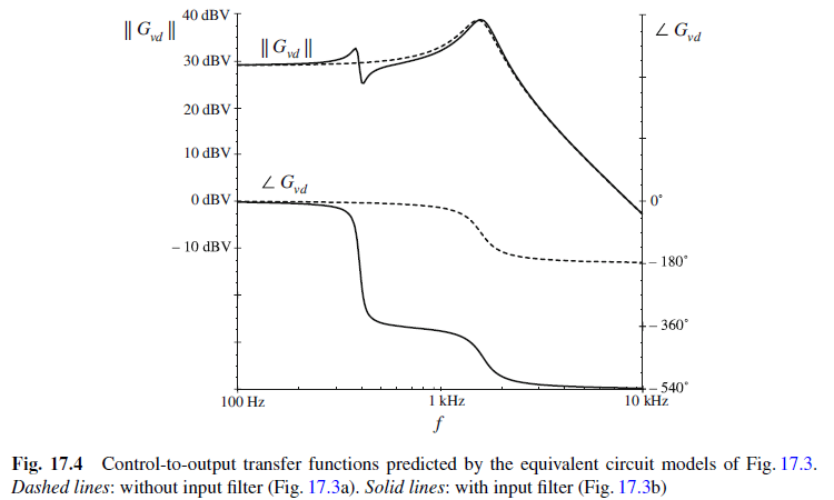
The Bode plot in the textbook is shown below. enter image description here
I used MATLAB to create a similar Bode response, using this code:

opts = bodeoptions;
opts.FreqUnits = 'Hz';

vd=5;
R=3;
D=0.5;
vo_desired=D*vd;
L=100e-6;
C=100e-6;
L_f=330e-6;
C_f=470e-6;


Gd0=vd;
w0=1/sqrt(L*C);
Q=R*sqrt(C/L);

Gvd=tf(Gd0,[1/(w0)^2,1/(Q*w0),1]);

Z=tf([L_f,0],[L_f*C_f,0,1]);
ZN=tf(-R/D^2,1);
ZD=tf([R*C*L,L,R],[C*R,1])/D^2;
Gvd_new=Gvd*((1+Z/ZN)/(1+Z/ZD));

bode(Gvd,opts,'r--')
hold on;
dcm = datacursormode;
dcm.Enable = 'on';
grid

bode(Gvd_new,opts)
legend('G_{vd}','G_{vd,new}')

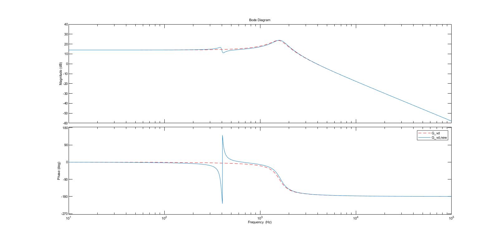
This results in this Bode: enter image description here

As you can see from the attached Bode plot I generated, the magnitude response seems to match what is shown in the textbook, but the phase response is significantly different. Am I missing something in my code or calculation?

\$\endgroup\$
5
  • \$\begingroup\$ A schematic of what the book plot represents is missing and, what your code represents has no schematic. \$\endgroup\$
    – Andy aka
    Commented Feb 7, 2023 at 11:16
  • \$\begingroup\$ The only obvious, big difference between the phase plots is phase unwrapping. The textbook "unwrapped" the phase, your Matlab plot didn't. \$\endgroup\$
    – JRE
    Commented Feb 7, 2023 at 11:46
  • \$\begingroup\$ @Andyaka apologies, the plots are for regular buck converters with an LC filter, I added the schematic. \$\endgroup\$
    – amidher
    Commented Feb 7, 2023 at 11:47
  • \$\begingroup\$ @JRE can you elaborate more please? what do you mean by unwrapping? \$\endgroup\$
    – amidher
    Commented Feb 7, 2023 at 11:50
  • 2
    \$\begingroup\$ The phase of the signal goes outside of -180 and 180 degrees in the textbook example. It ranges from 0 degrees to 540 degrees. Your example forces the phase to stay between -180 and 180 degrees. There's a discontinuity in you plot where the phase goes above 180 degrees and "wraps around" to -180 degrees. "Phase unwrapping" is used to make the phase continuous. Here's how you apply it in MATLAB. \$\endgroup\$
    – JRE
    Commented Feb 7, 2023 at 11:55

1 Answer 1

1
\$\begingroup\$

The general shape of your plot appears to match that of the textbook plot.

The biggest difference that I see is that the plot you made with MATLAB has a phase wrap-around while the textbook plot has the phase "unwrapped."

The MATLAB plot is constrained to stay between -180 and 180 degrees. That causes a discontinuity where the phase would exceed 180 degrees.

The textbook plot is continuous. It ranges from 0 to 540 degrees.

Your MATLAB program probably has "PhaseWrapping = 'on'" set in the "bodeoptions" somewhere. Since the default is "PhaseWrapping = 'off'", it must be your code that is turning it on.

\$\endgroup\$
1
  • \$\begingroup\$ Thank you so much, this might be an issue in the matlab version I am using, because i didn't anywhere in my code set the phase wrapping on. But that's ok fine, I just wanted to make sure I didn't make a mistake somewhere. Thanks again \$\endgroup\$
    – amidher
    Commented Feb 8, 2023 at 9:02

Your Answer

By clicking “Post Your Answer”, you agree to our terms of service and acknowledge you have read our privacy policy.

Not the answer you're looking for? Browse other questions tagged or ask your own question.