0
\$\begingroup\$

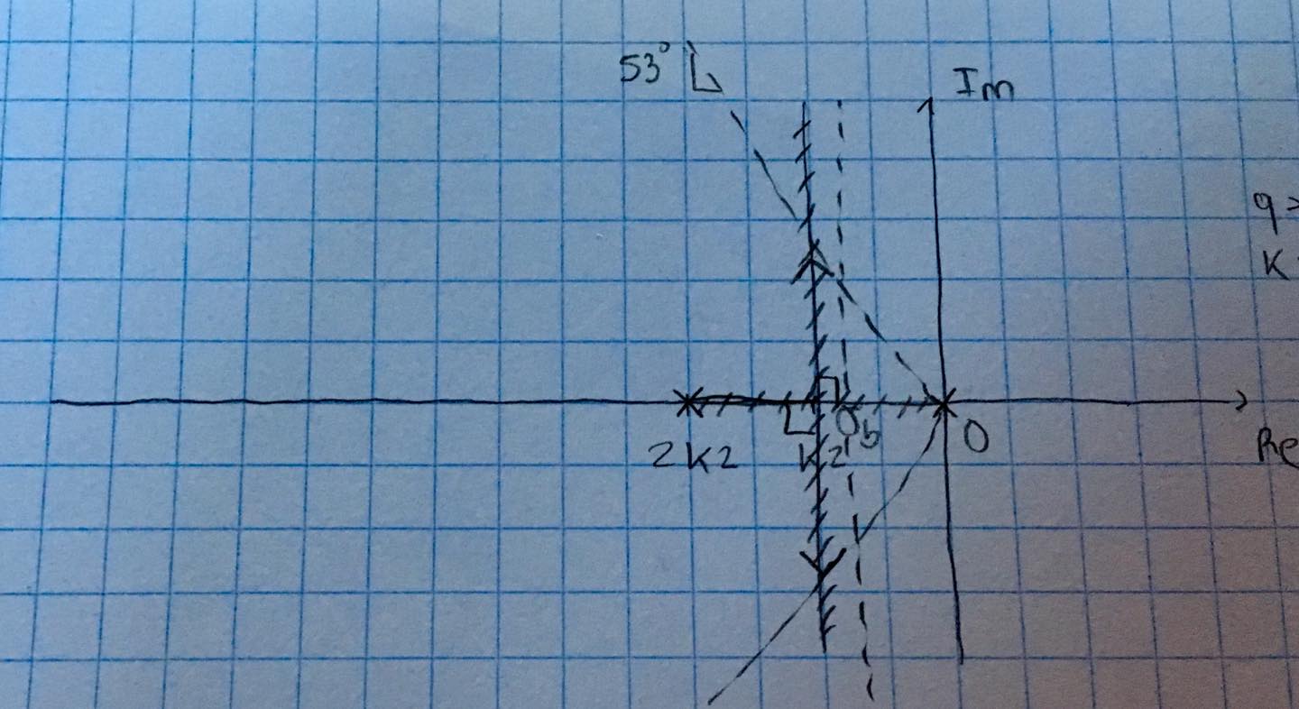
I want to find \$k_1\$ that leads to the feedbakc system having poles in the 53º line (to have overshoot \$\leq 10\%\$). From the root locus, the poles move along the vertical asymptote centered on -1. How can I find \$k_1\$ using Scilab and how can I draw diagonal lines representing the 53º line in which I want my poles to be at?

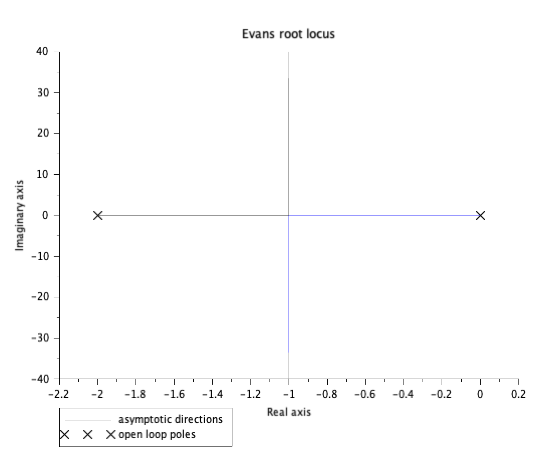
So far, I made this graph in Scilab,

Code:

s=%s;
num=2;
den=s*(s+2)
t=syslin('c',num/den);
clf;
evans(t);
mtlb_axis([-10 10 -2 2]);

Obtained graph:

enter image description here

Desired graph:

enter image description here

\$\endgroup\$
5
  • \$\begingroup\$ To draw the asymptotes there is a formula, web.calpoly.edu/~fowen/me422/RootLocus6.html \$\endgroup\$
    – jDAQ
    Commented Jan 10, 2020 at 18:44
  • \$\begingroup\$ @jDAQ I know the formula but I don't know how to implement it in Scilab. Could you help please? \$\endgroup\$ Commented Jan 10, 2020 at 18:51
  • \$\begingroup\$ I think that scilab is already doing it, but since the poles go along a line they go exactly over the asymptotes, try a third order system and you might see a difference in the asymptotes and pole path \$\endgroup\$
    – jDAQ
    Commented Jan 10, 2020 at 18:53
  • \$\begingroup\$ The axes must have the same scales if you're going to use geometry. \$\endgroup\$
    – Chu
    Commented Jan 10, 2020 at 19:11
  • \$\begingroup\$ @jDAQ the diagonal dashed line is given by overshoot, so the Scilab didn't draw this lines in the graph and I want to add to the graph manually. I want to know the intersection between root locus and the overshoot line to know the k of control system. \$\endgroup\$ Commented Jan 10, 2020 at 19:20

1 Answer 1

1
\$\begingroup\$

First, drawing two more lines with angles 53⁰ and -53⁰ should be easy, just do another plot while keeping the root locus. The lines should be, $$ y = \tan(53^\circ)x$$ and, $$ y = -\tan(53^\circ)x.$$

Once you have those lines, set some \$k\$ to be the maximum value of the evans function and change that value until you find the one that lies on the line you plotted. I would use a binary search to pick the values of \$k\$.

s=%s;
num=2;
den=s*(s+2)
t=syslin('c',num/den);
clf;

//test your k by changing this
k = 100;

evans(t,k);
mtlb_axis([-10 10 -2 2]);

//draw the 53 deg line
r = linspace(0,-3,10);
up_line = tan(53*%pi/180)*r;
dn_line = -tan(53*%pi/180)*r;
plot(r,[up_line; dn_line],'r-.')

//pzmap of the system with feedback
figure
plzr(1/.(t*k))

//draw the 53 deg line
r = linspace(0,-3,10);
up_line = tan(53*%pi/180)*r;
dn_line = -tan(53*%pi/180)*r;
plot(r,[up_line; dn_line],'r-.')

\$\endgroup\$
6
  • \$\begingroup\$ Thanks for help but the code in my computer crash in the line: plzr(1/.(t*k)) \$\endgroup\$ Commented Jan 10, 2020 at 21:48
  • 1
    \$\begingroup\$ it runs fine on my computer, try this, cloud.scilab.in \$\endgroup\$
    – jDAQ
    Commented Jan 10, 2020 at 21:54
  • 1
    \$\begingroup\$ You can also delete the code from figure downwards, that is just a pole-zero map, the root locus is done by the previous lines. \$\endgroup\$
    – jDAQ
    Commented Jan 10, 2020 at 22:12
  • \$\begingroup\$ Just to confirm: Scilab makes a 0 to infinity k scanner. If I want to make the k scanner from -infinity to 0, I need to add minus signal into the function numerator, right? \$\endgroup\$ Commented Jan 11, 2020 at 3:20
  • \$\begingroup\$ Yes, from zero to positive infinity \$\endgroup\$
    – jDAQ
    Commented Jan 11, 2020 at 3:29

Your Answer

By clicking “Post Your Answer”, you agree to our terms of service and acknowledge you have read our privacy policy.

Not the answer you're looking for? Browse other questions tagged or ask your own question.